
We all have atleast one story of how that one time the boss / co-worker / classmate / cat ruined the carefully crafted excel spreadsheet by mucking up the formulas or disturbing the formatting. There are 3 very easy solutions to prevent this problem,
- Write an unleash_a_pack_of_wild_cats_when_someone_messes_with_the_file () macro: It is not an elegant solution, and cats are not very consistent, but it can work.
- Move to marketing department, you dont need to send excel files any more, just ppts. 😛
- Or, read this post and learn 10 awesome tips on how to boss proof your excel files.
So here is the list of 10 tips to make better excel spreadsheets. I suggest using all these tips for a perfect boss proof workbook.
Restrict The Work Area Few Columns and Rows
Not all spreadsheets have 256 columns and 65000 rows of data. So why show the entire grid when you can, say, just show the 44 rows and 23 columns in which the sales report is presented.
To restrict the work area,
- Select the first column you dont want to see (24th column) and press CTRL+SHIFT+RIGHT ARROW. Now Right click and select “Hide” option.
- Select the first row you dont want to see (45th row) and press CTRL+SHIFT+DOWN ARROW. Now right click and select “Hide” option.
Lock Formula Cells And Protect The Worksheet
Formulas are the most vulnerable part of an excel sheet. You accidentally edit something, say in payroll sparesheet, and you just gave 3200% bonus to someone in the organization. That is alright if that someone is a CEO of a bailed-out bank, but in all other cases, you end up spending a sweet afternoon trying to figure out what went wrong.

So, it is better to lock the workbook formulas and protect the worksheet so that no one accidentally erase the formulas or mess with them. To do this follow the steps in the illustration above.
You can use the same trick to lock the charts and other worksheet objects.
Freeze Panes So that Your boss Knows what she is Reading

Freeze panes is a very useful feature. It locks the important items on the top so even when you scroll down you still see them. (You can do the same for columns, thus seeing the first few column even when scrolling left).
Bonus tip: Use excel tables (new feature in Excel 2007) so that you dont need to freeze panes. Learn more.
Hide Un-necessary / Calculation Sheets
It is fairly common for excel workbooks to have tens worksheets, some with data, some with calculations, some with intermediate stuff and only one or two sheets with actual outcome (like a dashboard or a report).

There is no reason to think that all these worksheets should be visible all the time to the boss. While it makes sense to have the data and calculations visible so that someone can audit the worksheet, I am sure you dont want your boss to waster her time doing that. So here is a handy tip:
- Select all the worksheets other than the output sheets and hide them.
Hide Rows / Columns
If for some reason, hiding worksheets is not possible, you can still try hiding rows and columns. This is a very good way to prevent someone from accidentally messing a with a row of “really big and complicated formulas”.

Just select the rows / columns you want to hide and right click and select the “hide” option.
Include Cell – Comments / Help Messages
We all know bosses have a busy mind. They dont have time to remember (or know) every little thing. Heck, sometimes they dont even know what somethings are.

I suggest using cell comments and help messages to give right information / guidelines to the spreadsheet end user, like “enter your age in this cell”. They are easy to implement and totally non-intrusive.
- To include a cell comment, select the cell and press SHIFT+F2 and write the comment.
To include a cell message, select the cell, go to data validation, go to “input message” tab and type what you want.
Data Validations, Error Messages
Spreadsheets are complicated things that are carefully crafted with umpteen pre-conditions and assumptions. I am sure there is at least one excel file out there that will only work if a cat enters the input. But we are not talking about cats, the point is, it is important that right data is fed to the worksheet before the formulas (or charts or payroll macro etc.) can work. That is where data validation can help.

It is very easy to set up data validation in excel. Just select the cell and go to data validation (in Data ribbon / menu). There are several ways in which you can set up data validations,
- You can show an incell drop down box and ask users to pick from a list
- You can specify the type of data allowed (dates, times, numbers, text)
- You can specify the length of data
- You can specify the conditions on data (like between 2 numbers, less than a given date etc.)
- You can even use formulas to make your own data validations [example]
There are several examples of using data validation in this site. Go check.
Use Consistent Colors And Schemes
Anything looks better when it is consistent, even when it is internally screwed up. That same rule applies to excel workbooks as well. It will make your boss feel comfortable and relaxed to see an excel workbook with consistent colors and (simple) schemes.
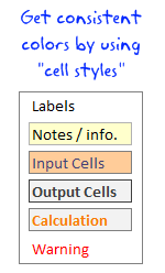
I suggest using excel cell styles to define the styles for your workbooks. This ensures consistency and you dont have to spend after hours formatting the worksheets. Read more about cell styles.
Name and Color Worksheet Tabs Appropriately
It doesnt matter if you have designed an awesome excel dashboard, your boss can be still pissed because the sheet name is “Sheet 69”. That brings us to the last and final point.

Use appropriate names (and may be tab colors) for the worksheet tabs. This makes the navigation easy and boss proof.
Learn how to color excel worksheet tabs.
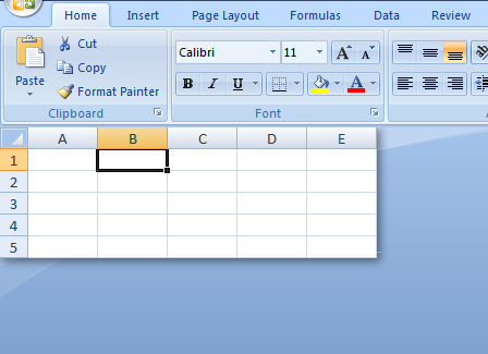
Before Closing The Workbook, Select Cell A1 On The Correct Sheet
Just before you finally save the workbook and e-mail it to the boss, make sure you are on the right worksheet (ie the dashboard or the report) and selected cell A1. The ensures that when the boss opens the workbook, she sees the right tab with right information, not some calculations or formulas.
That is all, you have just learned a handful of trick to impress your boss.
Share your boss proofing tricks for excel
Got an awesome idea that has been working on your boss? Share it with us in comments. I love to hear your stories and how you are using excel to further your career.
Be awesome, Learn few more excel tricks:
We at PHD have a simple goal – “to make you awesome in excel and charting”. Here is a list of articles I recommend reading if you are new here or just wanted to be more.
- 15 fun and exciting excel tips – who say spreadsheets are boring?
- 15 Excel formulas beyond IF() and SUM()
- 15 Excel productivity tips that you dont know
- 10 things about Excel 2007 that you should know to work better
- More articles on excel productivity
Dilbert cartoon from Dilbert.com


One Response to “Excel Tips Submitted by You [Part 4]”
ctl+d
copy the up cell