
Making charts is one of the most common use of Excel or other spreadsheet software. But do you know a simple trick that can save you lot of time while using excel charting features?
Chart Templates or User Defined Charts
yes, using chart templates can save you a lot of time.
If you use a particular type of chart or formatting all the time, you can save all the steps involved in making the chart by using templates.
Here is a simple tutorial on using chart templates in excel.
1. Prepare your chart
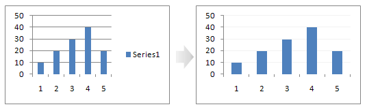
First step is to to prepare a chart that you would like to save to template. The chart can be a formatted version of one of the typical excel charts or a more complex combination chart.
2. Now save the chart as a chart template
 In excel 2007 you can do this by selecting the chart and going to design tab in the ribbon and clicking on “Save as template”
 For earlier versions of excel, right click on the chart and select chart type and go to “custom types” tab. Select “user-defined” as the chart type and click on the Add button to add the chart to excel chart templates.
3. Use the chart templates
Next time you need to insert a chart, use the templates and save time.

In Excel 2007 use the templates option. In earlier versions, use custom types to find your already save templates.
Bonus tip: Moving Chart Templates from One Computer to Another
If you want to move all your chart templates from one computer to another, just go to My Documents \Application Data\Microsoft\Excel and copy the file XLUSRGAL to the other computer. Make sure you are not overwriting the existing XLUSRGAL file, but just add the sheets from one file to another.
If you are using Excel 2007, the chart templates are stored as *.crtx files. Just locate them and copy to target system. Usually they can be found in \AppData\Roaming\Microsoft\Templates\Charts for Vista and My Documents \Application Data\Microsoft\Templates\Charts for XP.
Free Excel Chart Templates to Get you Started
And here is a huge list of beautiful excel chart templates, around 73 of them. Download and use them free. Get even more in our excel downloads page.
This is part of our Spreadcheats series, a 30 day online excel training series for office goers and spreadsheet users. Join today.


12 Responses
Hi, Does anyone else have any issues with these charts “collapsing”, condensing the data into a chart about 1cm tall??
@Ben.. I am not sure why this would happen. May be the templetized chart was saved like that… ?
I keep trying to use chart templates. The only thing it seems to apply is just the color/shape scheme. For example I have Titles, Value, Percentages and none of those are applied.
Additionally, I would like to further template the chart so that it automatically knows to make Wins = Green; Loss = Red; Pending = “Yellow” etc.
Anyway to do that?
Please send me a template on weekly sales /marketing
I would like my chart to automatically select the data, which is imported from a another program via a tab delimited text file.
The needed data always starts the same place (e.g. ‘A40’, ‘D40’ and ‘F40’ but there are differences in amount of data (typically a coupple thousands rows)
BR
/Daniel
Hey boy
Dear Chandoo,
I have prepared a 5 year projected balance sheet/CF/IS and other related working.
Now I want to prepare a graphical presentation using excel charts and then to prepare final presentation in powerpoint using worksheet and charts.
Can you help me how I can prepare the graphs and powerpoint presentation.
Appreciate your help, kindly reply to my above email.
Thanking you and best regards.
Aman
necesito mover un grafico a una hoja nueva pero que este grafico tenga como fondo el logo de la empresa detras de el grafico
Google Translate: I need to move a chart to a new sheet but this graph has as background the logo of the company behind the chart
Hello,
besides always wanting to say that “you are my Excel hero”, I am sure you have the answer to the following question:
is there any way to customize the Excel charts templates folder out of Appdata\Roaming\Microsoft\Templates\Charts … to, say d:\chart templates
I presume the answer is “sorry, can’t be done” but if somebody knows it would be you, right?
Best
Joe
The screenshots/directions to save the “free”templates do not seem to match up with my Excel 2010 version. Am I looking in the wrong place or were the templates written before v. 2010 release?
@Padean B
Chandoo.org has been around for a while
Chandoo started posting about Excel in 2008 well before Excel 2010 was around
The move to 2010 probably happened in 2011 and in 2014 we are now using 2013 as the base version.