Excel Links of the Week – Free E-Book Edition
blogging , excel links - 5 comments
 Good news!!! If you have been reading this blog for a while but haven’t yet joined the 2500+ reader community, here is a little incentive for you. When you sign up for our e-mail updates, I will send you the 95 excel tips so that you can rock between 9 to 5 e-book free. It is a 25 page ebook containing some of the best excel & charting tips posted in PHD in easy to read format.
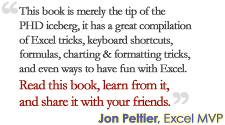
I have requested my friend and fellow Excel MVP, Jon to write a foreword for the book and he has been kind enough to some nice words about it, including:
And, if you are already a subscriber of PHD and would like to receive a copy of the book,
- send a blank e-mail to excelandcharting @ gmail.com
- with the subject: I want to rock between 9 to 5, send me the ebook
Ok, let us talk about this week’s excel links:
More Data Validation Goodness: Dynamic Ranges in Validation Lists
The problem: Validating data entry based on hierarchical (parent child) data. The example used is regions and countries but it could be countries and cities, product categories and sub-categories, class and student name, etc. You want to enter a region from a list of regions and in the next cell you want to select a country but only from the countries which belong to that region. How do you define the list of countries to validate against? The trick is basing the country validation list on an expression which will point to a different range based on the region value.
Import Delicious Bookmarks to Excel
Do you save a lot of bookmarks on delicious? Well, then this excel file can help you get a backup of all the bookmarks. It uses delicious api to fetch the bookmarks.
Excel date format conversion causes irrevocable damage to gentic research teams
When you enter a value like DEC-10 in an excel cell, it is automatically converted to date value. This can be a big problem if you want to use values like DEC-10 in a spreadsheet. Here is a simple workaround. First select the columns or rows where you want to enter values and press CTRL+1. Set the format from “Number” to “Text”. If only the genetic researchers used this little trick, it would have saved them lot of time.
A Robust String Concatenation Function
While the Concat VBA Function I have written can be used to concatenate a range of cells (along with a custom delimiter), it doesn’t accept arrays or multiple ranges as inputs. Chip Pearson has the perfect solution for you if you are looking for a string concatenation function that is more robust.
Two Simple things you should know to be a great presenter
Seth Godin pronounces 2 simple elements of a great presentation. We are all in the business of telling stories. Right from the moment we tell our story to the recruiter to the meeting you just attended, it is all about telling stories. And knowing how to present your ideas is very important. So …
If you have an excel link to share or just want to say hello
drop me a note at chandoo.d @ gmail.com or leave a comment. Have a fantastic week ahead everyone 🙂
PS: Photo from: http://www.flickr.com/photos/bearpark/2373643780/ by Memege a Moi

Hello Awesome...
My name is Chandoo. Thanks for dropping by. My mission is to make you awesome in Excel & your work. I live in Wellington, New Zealand. When I am not F9ing my formulas, I cycle, cook or play lego with my kids. Know more about me.
I hope you enjoyed this article. Visit Excel for Beginner or Advanced Excel pages to learn more or join my online video class to master Excel.
Thank you and see you around.
Related articles:
|
Leave a Reply
| « RSS Icon using Donut Charts – Because it is Weekend | How to use Excel Chart Templates and Save Time » |
 At Chandoo.org, I have one goal, "to make you awesome in Excel & Power BI". I started this website in 2007 and today it has 1,000+ articles and tutorials on data analysis, visualization, reporting and automation using Excel and Power BI.

5 Responses to “Excel Links of the Week – Free E-Book Edition”
Only one word: Superb!
Man I have never seen somebody so into Excel. You have to be either obsessive or borderline...
Anyway, good luck and I hope you make your tonnes of money frm this venture. Or at least try and get some link love from Microsoft for being so diligent in this xl macro sh*t.
No offense.
Hi Chandoo,
In your free ebook, the links to get the full tip are disabled. While saving it as pdf, you have not activated the links that are directed to your blog. Please check.
@Govert: thank you...
@Tarun: I am not obsessive. I am passionate about excel. I share what I learn and I find it very joyful. My aim is to use this blog as a platform to improve my teaching skills so that I can become a better teacher in real life. Of course, along the way I make some money due to all the ads etc. But the intention is not to make that money but to improve myself and help others in a small but meaningful way.
@Sumeet: Very good input. I didnt know the links were removed. I will try to release an update sometime during the next weeks.
Many thanks for the ebook, great reference!