
Imagine you are a carpenter and you are tasked with laying wooden floor at Gill Bates’ house. Now Gill B has a very big house and he wants to make sure you do a good job. So instead of asking you to lay the floor for entire house, he asks you to finish flooring in the guest bedroom first. Here are the dimensions of that guest bedroom.
- Width: 6ft 3inches
- Length: 24ft 9inches
- Size of individual wooden floor board: 2ft x 4inches
And here is the big question you are facing.
What?!? the guest bedroom width is only 6ft 3inches?
But over the years of chiseling and polishing you have learned to keep quiet and do your work.
So the real question you have is, How many wooden floor boards should you buy?
Of course, you want to find the answer using Excel. Why else would a carpenter read this blog?
Multiplying Feet & Inches using Excel
If the metric system became an universal standard for measuring things, we all can stop worrying and go to that wooden tile store to place order now. Alas, we still have to deal with feet, inches, miles, pounds, ounces and gallons (not to mention irrational numbers like pi, e and eleventeen).
Fortunately, Excel has 2 powerful features to support calculations like this.
Method 1: Using CONVERT()
CONVERT() as the name suggests is an Excel function that can convert values from one base to another, like feet to inches, square meters to square feet, centigrade to fahrenheit, grape juice to wine. Well, not the last one, but it shines in all other scenarios.
So we can use CONVERT() to first convert all the numbers to a common base like meters or inches or feet. Then perform the arithmetic. Once done, convert back to Feet & Inches.
Pretty simple eh?
See this model:
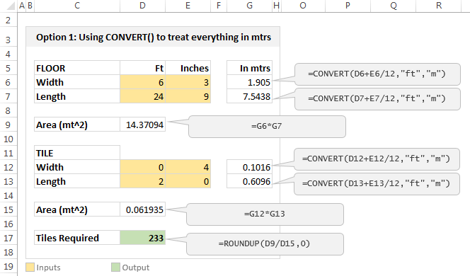
The process is simple:
- First we convert all feet & inch values to meters
- This is done with =CONVERT( feet value + inch value / 12, “ft”, “m”)
- Once we have values in meters, we perform the arithmetic by simple multiplication & division.
Method 2: Using Fraction Cell Format
If you don’t feel so hot for the CONVERT(), then this method works for you. You can use fraction cell formatting to enter fractions like 6 3/12 and 24 9/12 in to cells and let Excel treat them as regular numbers when multiplying, adding or dividing.
See this model:
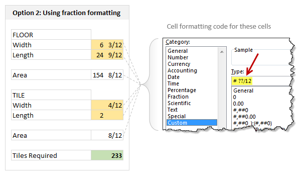
How to set it up?
- Select all the cells where you need values to be shown in feet inches fraction format
- Press CTRL + 1 (or right click and format cells)
- Select Custom and enter the formatting code as
- # ??/12
- This ensures that when you type a fraction like 6 3/12, Excel treats that as number (6.25)
- Rest of the arithmetic is simple.
Related: Custom Cell Formatting in Excel – Tips, more tips, even more tips
Bonus Tricks
Here are few more scenarios where you can use either CONVERT() or fraction formatting.
- If varnishing 1 square feet takes 2 minutes 30 seconds, how much times does it take to finish a 20 ft 6 in x 12 ft 9 in room?
- If average customer call lasts 3 minutes 10 seconds and Cynthia took 400 calls in last week, how many hours did she work?
- If Mr. Gill Bates earns $1000 per every 1 minute 4 seconds, how many days does it take for him to earn $10 million?
- How many teaspoons of honey per gallon?
Download example workbook:
Click here to download example workbook. It shows 3 methods for solving this problem. Examine the formulas and format settings to learn more.
Do you use Excel for these kind of problems?
I am not much of a carpenter. Few years ago, I decided to add a door to my office desk so that my kids (they learned how to crawl around that time) wouldn’t poke the reset button of my CPU. After buying necessary material (a wooden plank, nails, hinges, magnetic door locks) and wasting a day hammering nails in to my fingers, bending one of the hinges, almost breaking the wooden plank in to two, I gave up and closed the shelf-space completely instead (here is a pic of my carpentering disaster). So it suffices to say I do not use Excel for modeling my carpentry jobs.
But I am sure many of our readers are better carpenters, masons, plumbers, knitters or cooks than me. So tell me. Do you use Excel for modeling these kind of problems? What formulas, techniques and tips do you use? Please share using comments.
Now if you excuse me, I have to go look at the leaky faucet my wife is complaining about. I am sure I can ruin it with a pipe wrench.


25 Responses to “Shift Calendar Template – FREE Download”
Hi Chandoo,
your recent postings include only Excel 2007 templates. Unfortunately the company I work at still runs Excel 2003. Is it possible to get your awesome files in other excel version as well?
Thanks so much for your great excel stuff!
Is it possible to do this for shifts with hours instead of days? To organise a three shift day?
Thanks in advance,
Stelios
In my organization there are 45 employees i need split then into three shifts ex:A shift:14,B shift:14,C shift:14 and week off:3 kindly help me on this.
@Masthan
You need to understand what rules your company has for the various shifts / roster combinations
Chandoo, I once did a shift control spreadsheet for my team. I put one person in each line, the columns were the days. I put a shift code in each cell indicating in which shift that person should work, or if the person were out that day. I have two codes for being out. One is for vacations and one is to compensate days worked in weekends. This way I was able to count how many persons I have in each shift, how many were on vacations and how many were out compensating (that's the term we use here) weekend worked hours.
Later I included the possibility of a person be in two lines one for normal hours other for overtime. This is mainly used for planning purposes. If you would like I can send you an example. The only problem of this spreadsheet is that we don't have a person view, only this consolidated view.
Hi George, I would like to have a copy of your spreadsheet if you can share it.
Thanks in advance, Chuck
Hi Chandoo,
Where is the code located ? is it VBA ? If so , how do you hide it ? Or it is .NET ?
Thx
@Idan
.
No VBA or code, it is all done with Mirrors.
Only Joking,
.
But there is no VBA or code,
It is all done with Named Formulas and Lookups.
Have alook at the cells in the calander area and Named Formulas in the Formulas, Name Manager Tab.
How can i calculate between two or more different workbooks? Please, reply me as early as possible.
@Anand
Open the workbooks you want to link to
Start a formula = and click and change between workbooks as required.
You can use the View, Switch window menu to change workbooks mid formula
The format for using workbooks is
=[Workbook.xlsm]Sheet1!$A$1
or
=SUM('[Book2.xls]Sheet1'!$A$1:$D$10)
etc
Hi Chandoo,
I am working with a call centre wherein i ned to update at the month end 20 to 30 employees login hours which are defict to track it at the month end is very difficult is there any template which can be made to track that why on a particular day a guy who needs to be on calls was why not on calls.
Thank you so much Chandoo. This is really helping me. As usual, you rock.
What's FortyTwoDays and Calendar in Name manager?
Both are unused and FortyTwoDays doesn't make any sense.
I have a SQL db that contains records of events scheduled/completed on a particular date. Can this method ous building a calendar be used to display those events on the respective day?
Positively awesome!
I'm attempting to help a friend create a schedule for adult classes - and of course its not"paid help". Here is the scenario:
20 classes, instructor, room#, student class size, start date, number of class days (need to subtract weekends)
class
instructor
room
students
start
#days
PATH
karen
201
21
01/01/13
11
BILLING
jane
401
15
01/12/13
13
MEDISOFT
mike
301
11
01/25/13
9
he'd like to see these classes show up in different colors within the same month's calendar chart. He can draw it, but I'd like to see it done automatically through data, and I just can't visualize it, but I KNOW this will work - can you help?
Jan 🙂
Dear chandoo,
Try many way to download still can't access. Any way we want to try out 3 shifts with 3 guys in a group .eg Group A Morn, Group B Night and Group C Rest. And every each group must work on sunday to take turns. In fact we are security teams so that's why sunday is required to work. Pls guide and show how to put in the working calendar. Thank you in advance.
I've been trying to copy and/or recreate this to use in a workbook I'm doing for the transportation department I'm working for. I need to have the calendar on the first sheet in my document (it has graph's from data on another sheet). I'm trying to use it to track (with the conditional formatting) accidents and injuries. I've redone the conditional formatting to do 4 different accident types (no injury, near miss, OSHA recordable injury and work loss injury), but when I enter the formula's you have in the calendar portion where it says "DateOfFirst-FirstWeekDay" I can't figure out how you did that. Are you able to help?
I would like to use Excel to solve the following problem for a community work. I want to create a Driver schedule for a given month from a pool of volunteers for a community service. Each of these volunteers can drive only on specific days in a week. I would like to populate the driving schedule for each weekday with primary, secondary and tertiary drivers in a random fashion so that I do not overburden one person. I would greatly any help you can provide.
Hi chandoo,
Thanks for your valuable effort for create this template and let me know how to add multiple employees in the the Roaster.
Hi Chandoo,
This article on shift roaster is very helpful. Could you please let me know how i can use the same for n number of resources who work 24/7, considering their leaves and holidays?
Thanks,
Savitha
Hi Chandoo,
This article on shift roaster is very helpful to all. Could you please let me know how i can use the same if I want to add for some more shifts, since the color is not getting change if I add more shifts like 4,5 etc.,
Thanks,
Murali
nice post
How can I change the date to 2017 under Shift Data worksheet.
solution 1:
mydata=B2:C16
stoplist=E2:E8
=LET(RNG,A2:A16,SMR,C2:C16, F,(RNG=E2)+(RNG=E3)+(RNG=E4)+(RNG=E5)+(RNG=E6)+(RNG=E7)+(RNG=E8),SUM(SMR)-SUM(SMR*F))
=LET(RNG,A2:A16,SMR,C2:C16,RH,N(B2:B16=B2), F,(RNG=E2)+(RNG=E3)+(RNG=E4)+(RNG=E5)+(RNG=E6)+(RNG=E7)+(RNG=E8),TOT,SUM(SMR)-SUM(SMR*RH*F),SUM(SMR*RH)-SUM(SMR* RH*F))
ALTERNATE SOLUTION
=SUM(C2:C16)-SUM(FILTER(C2:C16,ISNUMBER(BYROW(A2:A16,LAMBDA(a,TOROW(SEARCH(a,E2:E8),2))))))
=SUM((B2:B16=B2)*(C2:C16))-SUM((ISNUMBER(BYROW(A2:A16,LAMBDA(a,TOROW(SEARCH(a,E2:E8),2))))*(B2:B16=B2)*(C2:C16)))
let
Source = Excel.CurrentWorkbook(){[Name="Table1"]}[Content],
#"Replaced Value" = Table.ReplaceValue(Source,null,";",Replacer.ReplaceValue,{"Column1"}),
#"Transposed Table" = Table.Transpose(#"Replaced Value"),
#"Removed Other Columns" = Table.SelectColumns(#"Transposed Table",{"Column1", "Column2", "Column3", "Column4", "Column5", "Column6", "Column7", "Column8", "Column9", "Column10", "Column11", "Column12", "Column13", "Column14", "Column15", "Column16", "Column17", "Column18", "Column19", "Column20", "Column21", "Column22", "Column23", "Column24", "Column25", "Column26", "Column27", "Column28", "Column29", "Column30", "Column31", "Column32", "Column33", "Column34", "Column35", "Column36", "Column37", "Column38", "Column39", "Column40", "Column41", "Column42", "Column43", "Column44", "Column45", "Column46", "Column47", "Column48", "Column49", "Column50", "Column51", "Column52", "Column53", "Column54", "Column55", "Column56", "Column57", "Column58", "Column59", "Column60", "Column61", "Column62", "Column63", "Column64", "Column65", "Column66", "Column67", "Column68", "Column69", "Column70", "Column71", "Column72", "Column73", "Column74", "Column75", "Column76", "Column77", "Column78", "Column79", "Column80", "Column81", "Column82", "Column83", "Column84", "Column85", "Column86", "Column87"}),
#"Merged Columns" = Table.CombineColumns(#"Removed Other Columns",{"Column1", "Column2", "Column3", "Column4", "Column5", "Column6", "Column7", "Column8", "Column9", "Column10", "Column11", "Column12", "Column13", "Column14", "Column15", "Column16", "Column17", "Column18", "Column19", "Column20", "Column21", "Column22", "Column23", "Column24", "Column25", "Column26", "Column27", "Column28", "Column29", "Column30", "Column31", "Column32", "Column33", "Column34", "Column35", "Column36", "Column37", "Column38", "Column39", "Column40", "Column41", "Column42", "Column43", "Column44", "Column45", "Column46", "Column47", "Column48", "Column49", "Column50", "Column51", "Column52", "Column53", "Column54", "Column55", "Column56", "Column57", "Column58", "Column59", "Column60", "Column61", "Column62", "Column63", "Column64", "Column65", "Column66", "Column67", "Column68", "Column69", "Column70", "Column71", "Column72", "Column73", "Column74", "Column75", "Column76", "Column77", "Column78", "Column79", "Column80", "Column81", "Column82", "Column83", "Column84", "Column85", "Column86", "Column87"},Combiner.CombineTextByDelimiter("|", QuoteStyle.None),"Merged"),
#"Split Column by Delimiter" = Table.ExpandListColumn(Table.TransformColumns(#"Merged Columns", {{"Merged", Splitter.SplitTextByDelimiter(";", QuoteStyle.Csv), let itemType = (type nullable text) meta [Serialized.Text = true] in type {itemType}}}), "Merged"),
#"Added Prefix" = Table.TransformColumns(#"Split Column by Delimiter", {{"Merged", each "|" & _, type text}}),
#"Replaced Value1" = Table.ReplaceValue(#"Added Prefix","||","|",Replacer.ReplaceText,{"Merged"}),
#"Split Column by Delimiter1" = Table.SplitColumn(#"Replaced Value1", "Merged", Splitter.SplitTextByDelimiter("|", QuoteStyle.Csv), {"Merged.1", "Merged.2", "Merged.3", "Merged.4", "Merged.5", "Merged.6", "Merged.7", "Merged.8"}),
#"Removed Columns" = Table.RemoveColumns(#"Split Column by Delimiter1",{"Merged.1"}),
#"Removed Duplicates" = Table.Distinct(#"Removed Columns")
in
#"Removed Duplicates"