
This is part 4 of 6 on Profit & Loss Reporting using Excel series, written by Yogesh
![Exploring Pivot Table Profit Loss Reports [Part 4 of 6]](https://chandoo.org/img/ea/profit-loss-report-pivot-options-4.png)
Data sheet structure for Preparing P&L using Pivot Tables
Preparing Pivot Table P&L using Data sheet
Adding Calculated Fields to Pivot Table P&L
Exploring Pivot Table P&L Reports
Quarterly and Half yearly Profit Loss Reports in Excel
Budget V/s Actual Profit Loss Report using Pivot Tables
This is continuation of our earlier post Adding Calculated Fields to Pivot Table P&L.
Now that we have P&L report as PivotTable, in this post we will explore excel features to make various types of reports.
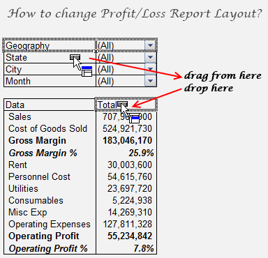
Making Reports by Geography / State /City or Month:
You can make Geography-wise , State-wise, City-wise or Monthly P&L with just few clicks. You just need to drop the required field to the column area of your PivotTable.
Want more? – You can prepare Geography wise P&L for the month of Dec.2009
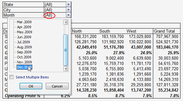
Keep exploring the power of Filters and use them in various combinations to make report on required parameters.
Making Report of Top 5 Stores based on a Parameter
Okay I have got something more for you, How about finding top five stores based on Gross Margin % or Bottom 5 Stores based on Operating Profit %
Add “Store” Filed to Column area of Pivot Table. Now right click on store filed > Click on Filters > Choose Top 10
Choose your options From Drop Down Menu

Above shows you to calculate Top 5 based on Gross Margin%, go ahead and try to find out Bottom 5 based on Operating Profits%
Define KPIs and Make Reports Based on them
By adding some more calculated fields you can calculate various KPIs from the same set of Data.
City wise KPI is just example , you can calculate them on any other parameter as we have done with PivotTable P&Ls above. Use these formulas to calculate these KPIs
Sales per SFT = Sales / ‘Store Area’
Rent per SFT = Rent / ‘Store Area’
Utilities per SFT = Utilities / ‘Store Area’
Consumable % = Consumables / Sales
Then you can prepare a KPI report like this:

Download Excel File with these Pivot Tables
Click here to download Explore PivotTable P&L.xls with these PivotTables [mirror].
What Next?
In the next part of this series, learn how to prepare quarterly and half-yearly profit loss reports in excel.
Meanwhile, make sure you have read the first 3 parts of this series – Data sheet structure, Preparing P&L Pivot Table, Adding Calculated Fields.
Also check out the Excel Pivot Tables – Tutorial, Pivot Table Tricks, Grouping Dates in Pivot Reports articles to get more ideas.
Added by PHD:
- Please share your feedback and ideas for this series using comments. Yogesh and I will reply to your questions. Also, say thanks if you like the idea and want to learn more.
- Sign-up for PHD E-mail newsletter because you will get updates as new posts are live.
 Yogesh is an accountant with 13 years of experience in India and abroad. His specialties are budgeting and costing, supplier accounting, negotiation of contracts, cost benefit analysis, MIS reporting, employees accounting. He writes about excel at http://www.yogeshguptaonline.com/


7 Responses to “Exploring Profit & Loss Reports [Part 4 of 6]”
Congrats Chandoo for your post.
I'm a fan of pivot tables for years, I really believe it’s the best invention since the copy / paste or the wheel, I would not know what is really best.
In your example you show geographical items and I was wondering if you can show this data with a map incrusted, I mean showing profits by cities, i.e.
What approach are you recommending?
Cheers!
Hi :
I'm accountant too...I know about pirvot table for alonge time. But I can't use it to do the inventory report that show movement about carry forward, receive , withdraw and balance for daily...Have anyone has a tip?
Mei hua
Thailand...
Social comments and analytics for this post...
This post was mentioned on Twitter by Excel_Insider: Exploring Profit & Loss Reports [Part 4 of 6]: This is part 4 of 6 on Profit & Loss Reporting using Excel series, ... http://bit.ly/9bVv06...
[...] Preparing Pivot Table P&L using Data sheet Adding Calculated Fields to Pivot Table P&L Exploring Pivot Table P&L Reports Quarterly and Half yearly Profit Loss Reports in Excel Budget V/s Actual Profit Loss Report using [...]
[...] Preparing Pivot Table P&L using Data sheet Adding Calculated Fields to Pivot Table P&L Exploring Pivot Table P&L Reports Quarterly and Half yearly Profit Loss Reports in Excel Budget V/s Actual Profit Loss Report using [...]
hi
I have data like:
Name Jan Feb March April total
bari 5 6 7 9 27
chand 5 3 2 10 20
narayan 7 3 8 6 24
in this date i want paviot table, Name is constant : and if i select any month i should get the partcular month with total, even if i select multi months i should get total of selected month data how can get this thro paviot
This is my first time creating a pivot table. I think I have been ok with lessons 1-3. At the start of lesson 4 I notice that the city, state month etc. have been added at the top of the pivot table. I must have missed something. How was this created?