
During one my recent training programs, a participant asked an interesting question.
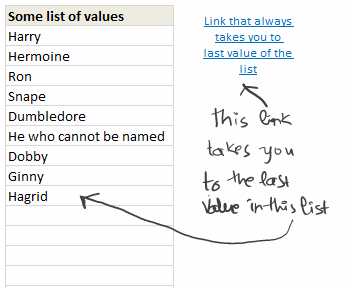
I have a list of values. I would like to place a hyperlink in my workbook that would always take me to the last value in the list.
Something like this,
Now, we all know that you can use HYPERLINK() function to create a hyperlink in Excel. Here is a detailed tutorial on hyperlinks in Excel.
But, how do we make the hyperlink dynamic?
Very simple, we just count how many values our list has and then link to the last cell’s address accordingly. See this video tutorial to understand how you can do it.
Dynamic Hyperlinks in Excel – Video Tutorial
Download Example Workbook on Dynamic Hyperlinks
Click here to download this example workbook. Play with it to understand how this technique works.
Do you use Hyperlinks? Share your tips
I use hyperlinks in my Excel workbooks all the time. They are easy to create and they make my workbooks more accessible. Adding a hyperlink is the easiest way to impress your audience.
What about you? Do you use hyperlinks? What are your favorite uses / tips? Please share using comments.
More Tutorials on Hyperlinks in Excel
Check out these tutorials to learn more about Hyperlinks in Excel
- Introduction to Excel Hyperlinks
- Creating a Table of Contents in Excel Workbook (and other tips)
- Creating a Birthday Reminder using Excel
- What is a Picture Link & How to use it?
PS: that is my hand-writing in the image above. I bought Genius Slim Tablet on my way back from Singapore. So I am playing with it.


43 Responses to “Create Dynamic Hyperlinks in Excel [Video]”
I never thought of using dynamic links, it makes generating hyperlinks so much easier and I might be more inclinded to use them.
I use hyperlinks for my own purposes of navigating a document, but find that other people just don't use them; they can use the internet, work complex machinery, but as soon as you put a number on a piece of paper, it's too much for them.....
Problem with hyperlinks is that they only work within the context of MS Excel. If you save the file as a "pdf" or print to a pdf the links are gone.
I use hyperlinks in workbooks containing data records, which are brought in from multiple source files. (To create such consolidated workbooks, I use Ron DeBruin's RDBMerge add-in).
To setup the hyperlinks I created a few macros which I've saved as a .bas module which can be imported into any workbook. If anyone's interested, I can send them the .bas file as a text file.
A couple of sample macros to create hyperlinks are given below.
1. This code runs through the cells in the current column and sets up a hyperlink to the filename in the active cell, until it encounters a blank cell. The code assumes that the cells contain valid FULL FILENAMES.
Sub CreateHyperlink_ActiveCellValue_LOOP()
Do While Not IsEmpty(ActiveCell)
ActiveSheet.Hyperlinks.Add _
Anchor:=Selection, _
Address:=ActiveCell.Value, SubAddress:="", _
TextToDisplay:=ActiveCell.Value
ActiveCell.Offset(1, 0).Select
Loop
End Sub
2. This code runs through the cells in the current column and sets up a hyperlink at for the first record of each filename. This code assumes that the active cell column is sorted by the filename (otherwise, each time the code encounters a different value in the next cell, it will create a hyperlink)
Sub CreateHyperlink_ActiveCellValue_FIRST_REC_LOOP()
' create a hyperlink to activecell value for
' each first record in the column
Application.ScreenUpdating = False
Do While Not IsEmpty(ActiveCell)
If ActiveCell.Offset(-1, 0).Value = ActiveCell.Value Then
ActiveCell.Offset(1, 0).Select
Else
ActiveSheet.Hyperlinks.Add _
Anchor:=Selection, _
Address:=ActiveCell.Value, SubAddress:="", _
TextToDisplay:=ActiveCell.Value
ActiveCell.Offset(1, 0).Select
End If
Loop
MsgBox "DONE!", vbInformation
End Sub
Interesting approach.
I personnaly like to use traditionnal hyperlink (CTRL+k) to a named range or cell.
That name could be dynamic or not.
Sébastien
Oh man, I know I have already plugged my rarely updated blog, but the latest article I wrote talks about using hyperlinks to create mouseover effects. That is by far my favorite use for hyperlinks.
Great! I have never use a dynamic hyperlink. Learn something new! 😉
That's a pretty nifty solution.
Chandoo, it isn't necessary to include a file name in the formula if you are linking cell from the workbook: =HYPERLINK("#sheet1!"&last_row,"Add new")
You can take a look at my workbook on the SkyDrive - it has more advanced hyperlink to jump to the top: https://skydrive.live.com/view.aspx?cid=D8C4BA5E02DC5FFB&resid=D8C4BA5E02DC5FFB%21255
Very cool and very practical tip Chandoo, thank you.
Viccaji thanks also for your comments. I would be interested to see your .bas file although I have to admit I don't what a .bas file is, is it like an add-in? I have used some of Ron's DeBruin’s macros to merge csv files and they have been fantastically useful.
Send to otherjack@yahoo.com
Cheers
John
In a previous position I used MS-Project for some major projects, but not everyone had a license, so I created a map of all the important data in MSP and hyperlinked to a shared excel file so everyone could see the latest project plans. I later linked sub projects to projects to project summaries, but beware, you have to open and close all the files from the bottom to ensure you get the updated value cascade to the top.
Hi Chandoo
I am yet to see the details, but if there is a gap in cells (if cell B13 & B14 are empty, and there is some detail in cell B17) then the hyperlink doesn't take to the last cell
Anshul
i tried to appply this "HYPERLINK" formula to labels on a chart. theorotically this seems like it should be possible since graph name labels will accept a reference formula. i have not been able to get it to work. any suggestions? getting any hyperlink formula to work within a graph would be nice, some VBA could set up the links to the series and then the graph could be dynamicly changed as a sort of drill down exercise.
If there are any Gaps in the list this modification will still work:
=HYPERLINK("[dynamic-hyperlink.xls]'dynamic hyperlink'!B"&MATCH("ZZZZZZZZZZ",B:B,1),"Link that always takes you to last value of the list")
Clever stuff! I can definitely see myself using this tip regularly. Thanks Chandoo!
[...] week we learned how to create dynamic hyperlinks in Excel. Today, I want to show you something even cooler. An interactive dashboard based on hyperlinks, [...]
I recently created a model for a client where I nested a VLOOKUP within HYPERLINK. This allows you to define the HYPERLINK path based on the data returned by the VLOOKUP.
@All.. thank you so much for the comments & love.
@Sebastien: Yes, named range based approach would also work the same. Plus it looks elegant.
@Oleksiy: Wow.. I didnot know that. Thank you so much for sharing it. Donut for you 🙂
@Clarity: Interesting use of HYPERLINK with VLOOKUP...
Hello,
if i have a column in the first excel sheet containing a list of table names and in the other sheets the fields and data of each of these table (1 table per sheet). the sheet names are the same as the table names in the first sheet.
How can i create a hyperlink dynamically so that when i click on one of the table names, i open the related sheet??
Regards,
Joe
Hi Chandoo,
I would like to know, how i can use hyperlink with my chart dynamically.Suppose i have bar chart and i want to hyperlink it with a picture so that whenever i click on any portion of my bar chart it shows me that picture.
Santosh
Hi Chandoo
I am trying to create a chart.I got inspiration for this chart from a link http://www.improving-visualisation.org/vis/id=137 . Please help in creating this kind of chart.
Santosh Tiwari
@Santosh
I would use the technique described here:
http://chandoo.org/wp/2011/04/13/how-to-make-a-5-star-chart/
Hi Hui,
Thanks for sending me link for hyperlink video.It was good one, but i am still wondering about how to create visualization which i had seen in http://www.improving-visualisation.org/vis/id=137 .
Satosh Tiwari.
@Santosh
Using the Coke Can example
So you make a Stacked Column Chart with 1 Column and 5 Stacked Series
Make a Coke Can outline with a white mask outside the Coke Can
Make a Coke Can and set the Opacity to about 40% (I Use CorelPaint or Paint.Net (Free) )
Place both pictures in front of the chart
Add other text and numbers to suit
Maybe pull this apart: https://www.dropbox.com/s/tffkx7g6uc9pfca/Coke.xlsx
Hi Hui,
Thanks a lot for sending me coke file.....i wonder how i can add link to different color section of coke.Please help me in this regard.
Santosh Tiwari
@Santosh
What do you mean by "Add link to different color sections"
The color sections of the chart are different series in a chart which is linked to your data
You can change the Label of the different series to link to something other than the Series value as is the case now
Hi Hui,
If you go through the link which i had provided you, you will find that on placing cursor on different color section, it will show different data outside of chart.I am trying to create vba for mouse over function and by using link and photo shoot technique i am looking to create that kind of effect in my visualization.
Santosh Tiwari
I have never done any work using a Mouse Over events:
There are references to them on the net like: http://peltiertech.com/WordPress/highlight-a-series-with-a-click-or-a-mouse-over/
One of the issues here is you now have a Coke Can in front of the chart, and so the chart won't have focus
Hi... I have been trying to develop a hyperlink that should have the following features....
the hyper-linked cell will show the name of workbook.
As I change the worksheet name hyperlink will remain same but update according to worksheet name.
If you have any tips for this, please provide me that....
@Safayet
When you say Change the Worksheet Name do you mean rename the current worksheet or change to a different worksheet?
@ Hui
Thank you for the concern... 🙂
I mean renaming the current worksheet. I want a hyperlink that will work even if I rename the worksheet.
@Safayet
This looks messy and it is but it works
=HYPERLINK("[Book1.xlsx]" & RIGHT(CELL("filename",Sheet2!A1), LEN(CELL("filename", Sheet2!A1))-FIND("]", CELL("filename", Sheet2!A1))) & "!B4","CLICK HERE")This will link to Sheet2 cell B4 in Workbook Book1.xlsx
Change the Workbook and Sheet name and Address name to suit
If you have any problems with it first I suggest you retype all the " manually as they sometimes get screwed up
@ Hui:
Thank You! It works.
I've entered this, but it only brings me to the first cell of the sheet...
=HYPERLINK("[nameoffile.xlsx]'sheename'!a"&(COUNTA(B:B)+1),"sheet note")
I'm not sure what I'm doing wrong. I want it to go to the last empty cell of the sheet in row A, but I've tried several things I've seen on this page and none want to work. I'm using Office Professional 2007. Can someone help me?
@LCO
The address needs to be as Text
so:
=HYPERLINK(ADDRESS(COUNTA(Sheet1!$B:$B)+1,1,,1,"[nameoffile.xlsx]Sheename"),"Sheet Note")Should do it.
Thanks so much!!! - the only problem now is if the worksheet has a space in the name of it it stops working. I've been looking for a solution online but can't find one that works.
@Lco,
Just in case you never found the answer to your question regarding a sheet with space(s) in it's name - here is the answer:
Suppose the sheets name, you are refering to - in the same Workbook - is: Sheet ABC
The following formula should work:
=HYPERLINK("#'Sheet ABC'!"&ADDRESS(COUNTA('Sheet ABC'!B:B)+1,1),"Type friendly name here")
Michael Avidan
“Microsoft®” MVP – Excel
ISRAEL
Question. Assume one is working with two defined names that are being tracked through out the worksheet - Male and Female. The user will reach one spreed sheet (lets call it sheet 1) that will have a cell that states "Click here". How could one design a simple formula for that cell that if the user clicked on it and the user was male (which is already known), another spreadsheet (Spreadsheet Male) would open with charts for a male and if female another spreadsheet (Spreadsheet female) would open with charts for a female. Tried creating a process whereby on a calculation page there is hyperlink for male (a1) and female (a2) and an if formula =if(sec="Male",a1, a2). a1 would contain a hyperlink to Spreadsheet Male and a2 would contain a hyperlink to Spreadsheet female. The only problem is that the formula will simply recognize the appropriate hyperlink but will not open the hyperlink. Is there any way to create an automatic opening of a hyperlink or a simpler way to do this. Thanks
@Chandoo,
Sorry for being so late 🙂
You don't need the File Name nor the Sheets Name if you only need to "Jump" to the lat value in column "B" in the same Sheet.
All you need is:
=HYPERLINK("#"&ADDRESS(COUNTA(B:B),2),"Go to last value in column B")
Michael Avidan
“Microsoft®” MVP – Excel
ISRAEL
Sorry for the TIPO. The formula should read:
=HYPERLINK("#"&ADDRESS(COUNTA(B:B)+1,2),"Go to last value in Column B")
Michael Avidan
“Microsoft®” MVP – Excel
ISRAEL
Dear,
I have a problem with my hyperlink in excel document register. It has corrupted.
Some numeric numbers are automatically added in the hyperlink address. Due to this reason when i click on the link the linked document is not open. But when remove thos numbers and click on the link it works fine.
Could you please help me to edit this link (in bulk) at once.
Thanks.
hello,
i have a request, am using excel to present information from my work and i have a problem.
i have this map and i want to create rollover effect : my idea is when my mouse is over a region 1 for example (without clicking) , some information will apears and if i go to region 2 that infomation will change . please help me
i will be appreciate if you could help me on that because am new in VBA.
i have a request, am using excel to present information from my work and i have a problem.
i have this map and i want to create rollover effect : my idea is when my mouse is over a region 1 for example (without clicking) , some information will apears and if i go to region 2 that infomation will change . please help me
i will be appreciate if you could help me on that because am new in VBA