Last week we learned how to answer questions like, “How many tiles in a room?” using Excel. We learned about CONVERT function and fraction number format settings in Excel.
But why stop at calculation? We can even model a room full of tiles, thanks to Excel’s grid nature.
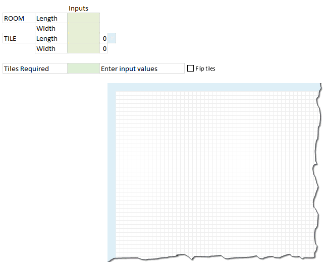
So today, we will learn how to create a room layout like this using Excel:

If you like the demo, read on to learn.
Step 1: Set up input cells
To model tiles in a room, we need 4 inputs. Lets call them by below names.
- room.length
- room.width
- tile.length
- tile.width
Step 2: Calculate number of tiles required
The basic formula for calculating total tiles required is this:
=ROUNDUP((room.length*room.width)/(tile.length*tile.width), 0)
But this formula yields in an unrealistic solution as we do not want to have fractional tiles everywhere. So, a better way to calculate this is,
=ROUNDUP(room.length / tile.length,0) * ROUNDUP(room.width / tile.width,0)
Although this formula is technically correct, you may save a few tiles if you rotate the them.
That is,
ROUNDUP(room.length / tile.width,0) * ROUNDUP(room.width / tile.length,0) can be smaller than ROUNDUP(room.length / tile.length,0) * ROUNDUP(room.width / tile.width,0) in some cases, as shown in above demo.
So we need a way to flip tile dimensions if that saves us a few bucks. That is done by,
Step 3: Flipping tile dimensions with a switch
Insert a check box and link to a blank cell, say F6.
[Related: How to use a check box in Excel]
Now, using F6 value (either TRUE or FALSE), flip the values of tile.length & tile.width using IF() formula.
Step 4: Create a 100×100 grid
Although you can model the floor plan of entire Buckingham palace in Excel, lets restrict ourselves to rooms of size 100×100.
Select 101 columns and resize them small enough so you can see all of them in a single screen, like 10 pixels wide.
Select 101 rows and adjust their height so that you can see as many of them as possible in a single screen (10 pixels tall should do).
Type running numbers in first column & row. The final grid looks this this:

Step 5: Modeling the room layout using conditional formatting
So we have a big 100×100 grid where we need to draw
- Outer boundary for the room as per room.length & room.width
- Inner tile boundaries as per tile.length & tile.width
Set up conditional formatting rules for room boundary
There are 4 rules required.
- Draw vertical left border if the topmost row = 1
- Draw vertical right border if the topmost row = room.length
- Draw horizontal top border if the left-most column = 1
- Draw horizontal bottom border if the left-most column = room.width
Below, see one of the rules.

You can find other conditional formatting rules in the downloadable workbook.
Step 6: Modeling Tiles using conditional formatting
While we need 4 rules for the room boundary, we just need 2 rules for tile boundaries.
- Draw vertical right border if the topmost row value is divisible by tile.length
- Draw horizontal bottom border if the left-most column value is divisible by tile.width
We do not need rules for vertical left border or horizontal top border because they will be drawn by previous tile.
See one of the rules below:

That’s all. Our room model is ready. Go ahead and see how it looks when tile it.
Download Example Workbook
Click here to download room tiles model workbook and play with it. Examine the conditional formatting rules to understand it better.
Do you apply Conditional Formatting in such creative ways?
I personally think conditional formatting is as good as honey, mangoes or dark chocolate. I love to use a dollop of it in all my Excel recipes.
What about you? Do you use conditional formatting for anything out-of-box 😉 like this? Please share your tips using comments.
Want more? Check out these conditional formatting examples
If you want more on conditional formatting you are in luck. Check out,
- Gantt chart using Excel conditional formatting
- Baby feeding schedule using conditional formatting
- Todo list using Excel conditional formatting
- Making data entry forms awesome with conditional formatting
- Searching data using conditional formatting
- Market segmentation charts with conditional formatting
- More examples on conditional formatting


40 Responses to “Looking up when the data won’t co-operate (case study)”
Nice Trick.. Clever use of cell references
Here is a formula I tried to create:
=SUMPRODUCT(((NOT(ISERROR(SEARCH(L5,B4:H14))))*1),(B5:H15))
It takes care of Caveat #1 (can handle text), but Caveat #2 remains.
In situations like this, I will often use VBA to restructure the data (2 columns: dates and values) on to a new worksheet. I can then use this 'clean' source for data analysis (formula or pivot table).
=SUMPRODUCT(((NOT(ISERROR(SEARCH(L5,B4:H14))))*1),(B5:H15)) and complex formulae in general are all very well but when you come back to them in a few weeks / months time, it is not at all easy to see what they do and what the limitations are.
Hi Chandoo,
I had used this type of cell ref. various times while calculating average.
But for the situation here try below formula . Note this is an array formula and must be confirmed with Ctrl+Shift+Enter.
=SMALL(IF(MMULT((L5=B4:H14)*IF(ISNUMBER(B5:H15),B5:H15),{1;1;1;1;1;1;1}),MMULT((L5=B4:H14)*IF(ISNUMBER(B5:H15),B5:H15),{1;1;1;1;1;1;1})),1)
Regards,
Hi, I think Using SEARCH in here will create a problem say there is a text like SUN and another text SUNLIGHT both result will be added by SUMPRODUCT.
Regards,
Array option.
=SUM(IF(MOD(ROW(B4:B14),2)=MOD(ROW(B4),2),IF(B4:H14=L5,B5:H15)))
Regards
@Elias,
Nice approach.
Although not requested - the formula I suggested closes all possibilities.
Criteria: _____ Value to retrieve:
Date__________ Numeric
Date__________Textual
Textual________Numeric
Textual________Textual
While your formula copes with only the 3 first combinations.
Michael (Micky) Avidan
“Microsoft® Answer” – Wiki author & Forums Moderator
“Microsoft®” MVP – Excel (2009-2015)
ISRAEL
@Michael,
Sorry but I don’t understand your point. I believe the challenge was to return the summary of a given date. What is your really volatile formula doing that mine is not?
Regards
@Elias,
I didn't say that the challenge differs from what you just mentioned/aimed to nor that your formula doesn't provide the requested result.
Please read my previous comment again and focus on the last combination (TEXT / TEXT).
I, myself, always try to provide a global Formula that is capable to handle all sorts of data.
Michael (Micky) Avidan
“Microsoft® Answer” – Wiki author & Forums Moderator
“Microsoft®” MVP – Excel (2009-2015)
ISRAEL
@Michael,
I see your point, but you are missing the below points if you are trying to cover all sorts of data.
What happened if the lookup value does not exist?
Do you want the first, second, summary, concatenation of the values if the look value is repeated?
See they are too many possibilities to be cover with just one formula.
Regards
1) The range: B4:H15 was named: RNG.
2) The following Array Formula was "retrieved from my sleeve" and I hope it can be shorten.
3) The formula seems to take care of BOTH(!) caveats.
-------------------------------------------------------------------------------
=OFFSET(INDIRECT(ADDRESS(SMALL(IF(RNG=L5,ROW(RNG),""),1),MOD(SMALL(IF(RNG=L5,(ROW(RNG))+COLUMN(RNG)/10),1),1)*10)),1,)
-------------------------------------------------------------------------------
Michael (Micky) Avidan
“Microsoft® Answer” – Wiki author & Forums Moderator
“Microsoft®” MVP – Excel (2009-2015)
ISRAEL
@Michael,
Check what happened with your result if you type 41927 in D5.
Regards
Correct. Didn't predict that.
Will find time to work something out.
Michael (Micky) Avidan
“Microsoft® Answer” – Wiki author & Forums Moderator
“Microsoft®” MVP – Excel (2009-2015)
ISRAEL
@Elias,
Let's hope the following Array Formula "closes all open doors".
Again - it has nothing to do with your formula which works fine as long as the 3 first mentioned combinations are concerned.
-------------------------------------------------------------------------------
=INDEX(RNG,LARGE(IF(RNG=L5,MOD(ROW(RNG)-1,2)*(ROW(RNG)),""),1)-2,(MOD(SMALL(IF(RNG=L5,(ROW(RNG))+COLUMN(RNG)/10),1),1)*10)-1)
-------------------------------------------------------------------------------
Michael (Micky) Avidan
“Microsoft® Answer” – Wiki author & Forums Moderator
“Microsoft®” MVP – Excel (2009-2015)
ISRAEL
Ok, if you insist. The following will cover all the scenarios you listed. However, I’ll never recommend/use such of formula.
Defined names:
rDat = $B$4:$H$15
rRow =ROW(rDat)-MIN(ROW(rDat))+1
rCol =COLUMN(rDat)-MIN(COLUMN(rDat))+1
rInc =MOD(rRow,2)=MOD(MIN(rRow),2)
L6=INDEX(rDat,MAX(IF(rInc,IF(rDat=L5,rRow)))+1,MAX(IF(rInc,IF(rDat=L5,rCol))))
Array Enter
Regards
@Michael,
unfortunately, your array formula still seems to return wrong results (eg 3-Nov).
If data are organized like in the example, ie. looks like a calendar, the INDEX formula seems quite simple:
=INDEX($B$4:$H$15,ROUNDDOWN((L5-B4)/7,0)*2+2,MOD((L5-B4),7)+1)
Yours is effectively the same as what I just came up with, and I believe this is the optimal answer to this particular problem.
My solution, before I saw yours:
=OFFSET(B5,QUOTIENT(L5-B4,7)*2,MOD(L5-B4,7))
OFFSET will work for an arbitrary list size, but INDEX might be easier to read.
QUOTIENT does the round and division in a single step.
If there's an improvement over Elias's solution then I for one can't see it.
Perhaps a non-CSE version which would also mean that only two references (B4:H14 and B5:H15), as opposed to three (B4, B4:B14 and and B5:H15), would require manually amending should the data range change, i.e.:
=SUMPRODUCT((ISEVEN(ROW(B4:H14)-MIN(ROW(B4:H14)))*(B4:H14=L5)*B5:H15))
I suppose we could make it a single, uniform range reference:
=SUMPRODUCT((ISEVEN(ROW(B4:H14)-MIN(ROW(B4:H14)))*(B4:H14=L5)*OFFSET(B4:H14,1,,,)))
which might be more appropriate should we e.g. wish to use a Defined Name for our range, i.e.:
=SUMPRODUCT((ISEVEN(ROW(Rng)-MIN(ROW(Rng)))*(Rng=L5)*OFFSET(Rng,1,,,)))
though whether that compensates for the extra, volatile function call is something to be debated.
Regards
I have tried something and then my Excel workbooks got shut down. Maybe that was too much?
Anyway here is what I've tried:
=SUMPRODUCT(INDEX(B5:H15;IF(ISEVEN(ROW(B5:H15));ROW(B5:B15)-ROW(B5)+1);{1\2\3\4\5\6\7}))
Guess that was wrong? Would this approach work anyway?
Looking forward to learn something from you Excel Experts.
Sorry, I haven't took notice of XOR LX's answer. I guess that's kind of what I was looking for.
@Michael Avidan
As it stands that is not a very rigorous construction.
You say "I, myself, always try to provide a global Formula that is capable to handle all sorts of data", which is a wonderful philosophy, but isn't it at least as important that we ensure that our formulas are independent of the row and column references of the data range in question, so that, should that range change, we do not have to re-work our solution?
What happens with your formula, for example, if RNG is instead re-located one row down, from B4:H15 to B5:H16?
When a formula is reliant upon the addition/subtraction of certain constants within the formula, which themselves are necessarily dependent upon the specific rows/columns in which the data lies at any given time (e.g. the -1 in MOD(ROW(RNG)-1,2)), then that formula is not a very flexible one.
Hence the reason for my choice of a slightly longer construction:
ROW(B4:H14)-MIN(ROW(B4:H14))
which ensures that this part of the calculation is not dependent upon the precise location of the data range within the worksheet, and so will give correct answers even if that range is re-located.
Regards
{=OFFSET(B4,MAX((B4:H15=L5)*ISODD(ROW(1:12))*ROW(1:12)),MAX((B4:H15=L5)*ISODD(ROW(1:12))*COLUMN(A:G))-1)}
Non-array formula:
=INDEX(B4:H15,SUMPRODUCT((B4:H15=L5)*(ROW(B4:H15)-ROW(B4)+1)*ISODD(ROW(B4:H15)-ROW(B4)+1))+1,SUMPRODUCT((B4:H15=L5)*(COLUMN(B4:H15)-COLUMN(B4)+1)*ISODD(ROW(B4:H15)-ROW(B4)+1)))
Using one range (B4:H15), one reference (B4), one lookup value (L5) and no INDIRECT or OFFSET.
My trial with defined names:
DateRange
=$B$4:$H$4,$B$6:$H$6,$B$8:$H$8,$B$10:$H$10,$B$12:$H$12,$B$14:$H$14
Position
=RANK('lookup problem'!$L$5,DateRange,1)
L6
=OFFSET(B4,ROUNDUP(Position/7,0)*2- 1,IF(MOD(Position,7)=0,6,MOD(Position,7)-1))
I'd probably just run with something like:
=SUMPRODUCT((B4:H14=L5)*(MOD(ROW(B4:H14),2)=MOD(ROW(B4),2))*B5:H15)
...which is basically the same as Elias' but without the IFs
The opposite of elegant but it works...
=INDEX(B4:H15,IFERROR(MATCH(L5,B4:B14,0),0)+IFERROR(MATCH(L5,C4:C14,0),0)+IFERROR(MATCH(L5,D4:D14,0),0)+IFERROR(MATCH(L5,E4:E14,0),0)+IFERROR(MATCH(L5,F4:F14,0),0)+IFERROR(MATCH(L5,G4:G14,0),0)+IFERROR(MATCH(L5,H4:H14,0),0)+1,IFERROR(MATCH(L5,B4:H4,0),0)+IFERROR(MATCH(L5,B6:H6,0),0)+IFERROR(MATCH(L5,B8:H8,0),0)+IFERROR(MATCH(L5,B10:H10,0),0)+IFERROR(MATCH(L5,B12:H12,0),0)+IFERROR(MATCH(L5,B14:H14,0),0))
=INDEX(B4:H15,
IFERROR(MATCH(L5,B4:B14,0),0)+
IFERROR(MATCH(L5,C4:C14,0),0)+
IFERROR(MATCH(L5,D4:D14,0),0)+
IFERROR(MATCH(L5,E4:E14,0),0)+
IFERROR(MATCH(L5,F4:F14,0),0)+
IFERROR(MATCH(L5,G4:G14,0),0)+
IFERROR(MATCH(L5,H4:H14,0),0)+1,
IFERROR(MATCH(L5,B4:H4,0),0)+
IFERROR(MATCH(L5,B6:H6,0),0)+
IFERROR(MATCH(L5,B8:H8,0),0)+
IFERROR(MATCH(L5,B10:H10,0),0)+
IFERROR(MATCH(L5,B12:H12,0),0)+
IFERROR(MATCH(L5,B14:H14,0),0))
Named Range
rownum = SUMPRODUCT(('lookup problem'!$B$4:$H$14='lookup problem'!$L$5)*ROW('lookup problem'!$B$4:$H$14)*ISEVEN(ROW('lookup problem'!$B$4:$H$14)))
Formula
=OFFSET($A$1,rownum,MATCH(L5,INDIRECT("$B"&rownum&":$H"&rownum),0))
How about SUM(IF(B4:H14=L5,B5:H15)) with array..it should work
Sorry, Chandoo, you can't find stuff this way in every possible scenario.
What if 2014-10-01 sales would equal 41.927 ? Which is serial number for 2014-10-15 ? SUMIF would fail to retrive correct answer. And your example data suggest that such number is possible in your table.
It's better not to search through dates and numbers at the same time.
If I'd solve a problem like this, it'd reformat table first so I get one column with dates and the other with numbers.
In this case, formula to form date column would be:
=INDIRECT(ADDRESS((INT((ROW()-4)/COUNT($B$4:$H$4))+1)*2+2;MOD(ROW()-4;COUNT($B$4:$H$4))+2;4;1))
and numbers would be the same formula with sight adjustment (+3 instead of +2 at the end of first argument):
=INDIRECT(ADDRESS((INT((ROW()-4)/COUNT($B$4:$H$4))+1)*2+3;MOD(ROW()-4;COUNT($B$4:$H$4))+2;4;1))
And now you got two columns that you can safely use for searching!
Oops, sorry, you actually mentioned that it doesn't work if number=date! I missed that part 🙁
={OFFSET(A1,SUM((B4:H14=L5)*ROW((B4:H14))),SUM((B4:H14=L5)*COLUMN((B4:H14)))-1)}
Works for all data... the solution I got for indirect looks little lengthy
I want to count last 20 records of a person, whose marks is greater than 2 and grade "manager". ....
Assume A1 has got names (James, John...etc...)
A2 "Manager"
A3 "2"
Someone please reply
I want to count last 20 records of a person, whose marks is greater than "2" and grade "Manager"
Assume A1 "geroge" A2 "Michael" A3 "George" etc...name can found anywhere in the rows
B1 "Manager" B2" clerk"
C1 "2" C2, "4"
please reply
Simplest I can come up with. No limitations for either 1 or 2. This does assume dates are an ordered list with 7 per row, and 2 rows per set. Assuming this is always true this will work for an arbitrary long list of dates.
=OFFSET(B5,QUOTIENT($L$5-$B$4,7)*2,MOD($L$5-$B$4,7))
@Marc,
Nice approach - however, as there are no "Negative Dates" - try:
=OFFSET(B5,INT(L5-B4)/7)*2,MOD(L5-B4,7))
——————————————————————————-
Michael (Micky) Avidan
“Microsoft® Answer” – Wiki author & Forums Moderator
“Microsoft®” MVP – Excel (2009-2015)
ISRAEL
=OFFSET(B4,ROUNDUP((L5-41911+1)/7,0)*2-1,MOD(L5-41911,7))
B4 has been used as reference cell for OFFSET().
FOR ROWS:
ROUNDUP(....,0) gives the integer value of a division. In case of presence of a remainder, ROUNDUP will add 1 to the Quotient.
As opposed to ROUNDUP(), the INT() or QUOTIENT() functions eliminate the remainder.
41911 = 01-Sept-2014, the first date in the data.
*2 has been used because there are 2 columns per set of data.
/7 has been used because there are 7 columns per set of data.
For columns
MOD(L5-41911,7))
Vijaykumar Shetye,
Panaji, Goa, India
This is how i did it
{=INDEX(B4:H15, MAX((L5=B4:H15)*ROW(B4:H15))-2, MAX((L5=B4:H15)*COLUMN(B4:H15))-1 )}
Here's my solution:
=INDEX(B4:H15,MATCH(1,MMULT(--(B4:H15=L5),TRANSPOSE(COLUMN(B4:H15)^0)),0)+1,MATCH(1,MMULT(TRANSPOSE(--(B4:H15=L5)),ROW(B4:H15)^0),0))
Sorry, forgot to mention Ctrl Shift Enter is needed.