How to transpose a values in a row to column using formulas… [Quick tip]

Share

Facebook
Twitter
LinkedIn

This is interesting, I am in Columbus to meet one of my college friends. I remember him as a very meticulous person from college days. So it is no surprise when he showed me his massively impressive finance tracker last night. He has been tracking expenses, income, credit card payments and gas (petrol) consumption since 2008. Very impressive indeed.

Then out of blue he said, he has a problem with his spreadsheet. In this own words,

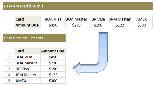
When entering data for credit cards, I use one column per card. But in my report view, I want to show credit card details in rows. How do I do this?

Something like this:

How to transpose a values in a row to column using formulas...

Transposing values in a row to column using formulas

If it is a one time process, my friend can use Paste Special > Transpose feature and be done. But this is no one time business. So lets understand which formula helps us do this.

  1. Lets assume original data is in $F$4:$J$5. Row 4 has card names & Row 5 has amounts.
  2. Wherever you want the out put, just list running numbers (1,2,3….) in a column. Lets say these are in cells D10:D14.
  3. To get the first card name, you can use the formula =INDEX($F$4:$J$4, $D10)
  4. To get the first amount due, use the formula =INDEX($F$5:$J$5, $D10)
  5. Now drag both these formulas down and you are done!

This is good, but I don’t like the extra column…

If that is the case, you can use the ROWS() formula to generate these running numbers for you on the fly. For example,

=INDEX($F$4:$J$4, ROWS($A$1:A1)) would work perfectly.

Learn more about: using ROWS / COLUMNS formula to generate running numbers.

Play with this formula

See the embedded Excel workbook below. Play with the formula.

(alternatives: download the example file or view it online)

How do you transpose values?

I love using INDEX formula. I use it for transposing values, tables, getting a cell value (or reference) from a large table, use it along with MATCH etc. It is a very versatile formula and I keep learning new uses for it.

What about you? Do you transpose values often? What formulas do you use? Please share using comments.

More on transposing your data:

If you like to transpose, wrestle or arm twist your data often, then you are at right place. Chandoo.org has tons of tutorials, material and tricks on this. Start with these:

Also, check out more quick tips.

Facebook
Twitter
LinkedIn

Share this tip with your colleagues

Excel and Power BI tips - Chandoo.org Newsletter

Get FREE Excel + Power BI Tips

Simple, fun and useful emails, once per week.

Learn & be awesome.

Welcome to Chandoo.org

Thank you so much for visiting. My aim is to make you awesome in Excel & Power BI. I do this by sharing videos, tips, examples and downloads on this website. There are more than 1,000 pages with all things Excel, Power BI, Dashboards & VBA here. Go ahead and spend few minutes to be AWESOME.

Read my storyFREE Excel tips book

Overall I learned a lot and I thought you did a great job of explaining how to do things. This will definitely elevate my reporting in the future.
Rebekah S
Reporting Analyst
Excel formula list - 100+ examples and howto guide for you

From simple to complex, there is a formula for every occasion. Check out the list now.

Calendars, invoices, trackers and much more. All free, fun and fantastic.

Advanced Pivot Table tricks

Power Query, Data model, DAX, Filters, Slicers, Conditional formats and beautiful charts. It's all here.

Still on fence about Power BI? In this getting started guide, learn what is Power BI, how to get it and how to create your first report from scratch.

23 Responses to “Displaying Text Values in Pivot Tables without VBA”

  1. sam says:

    Its possible to display up to 4 text values.

    Have a look at the screen shot of an example that I had posted way back at the EHA and figure out how its done !

    http://tinypic.com/r/muzywk/6

  2. ruve1k says:

    With Excel 2010 you can use Conditional Formatting to apply custom number formats which can display text. (In older versions you can only modify text color and cell background color, but not number formats.) Using CF allows for an even larger number of different display values.

  3. soumya says:

    Hey,
    Thanks, this helps. But how do you do it for multiple values where there is a huge amount of non repeating  text? 

  4. [...] Pivot Tables take tables of data and allow the user to summarise and consolidate the data at the same time. This is a great and very fast method of analysis but is restricted to handling mathematical functions on the value field resulting in numerical summaries. – read more [...]

  5. […] Read more here: Displaying Text Values in Pivot Tables without VBA […]

  6. Jon Gali says:

    There is a very good way actually for handling text inside values area.
    First you create a special column on the very left side and call it ID, and put unique ID (numbers only), and then create a pivot table with:

    Row Labels and Column labels as you like, and in the Values labels use the unique ID number.

    Move the unique ID number (copy paste) somewhere to the right and use vlookup to load the data you need using the ID as reference.

    It is a bit longer way but for me it works perfectly to combine values as you like in any moment.

    hope helps.

    Regards,

    Jon

  7. Linda says:

    Thank you! I finally understand pivot tables thanks to your clear, concise explanations and examples.

  8. Danzi says:

    Good Day. This is exactly what i have been looking for. However when i try it on my pivot table or even when i try to recreate this exercise using the sample worksheet, i get this error:

    "Microsoft Excel cannot use the number format you typed. Try using one of the built-in number formats."

  9. Hiren says:

    pls. help in table there is name, pan. amount. i have to make pivot table for example
    NAME PAN AMOUNT
    MR.X AAAAC1254T 500.00
    MR.Y AAABR1258C
    MR.A CFVDE2458T
    MR.Z AAVCR12548C
    MR.X AAAAC1254T
    MR.Z AADCD245T

  10. Hiren says:

    pls. help in table there is name, pan. amount. i have to make pivot table for example
    NAME PAN AMOUNT
    MR.X AAAAC1254T 500.00
    MR.Y AAABR1258C 1000
    MR.A CFVDE2458T 2000
    MR.Z AAVCR12548C 5451
    MR.X AAAAC1254T 45564
    MR.Z AADCD245T 4500
    how to get pivot tabe so i get PAN no. against Name.

  11. Letitgo says:

    I found an easy way to get text values in pivot table.

    I create an other worksheet in wich each cell has a formula that copy the pivot table. The trick is that the formula does a lookup for the numbers in the pivot table.

    The formula looks like that:
    =IF(ISNUMBER(table!A1);VLOOKUP(table!A1;Code!$A$1:$B$65;2);IF(ISBLANK(table!A1);" ";table!A1))

    Code is a worksheet where there is a liste of text /numbers correspondance.

    As a bonus The new sheet is easier to format

    Additional trick:
    In my case, i encoded differents codeid with a power(2, codeId-1) so that summing then is equivalent to concatenate them.

    1-A
    2-B
    4-C
    8-D

    yields :

    5 - AC
    14 - BCD

  12. Tushar says:

    Hi
    I want to ask if pivot can display dates in pivot field. As in a column i have customers and in row different items i want to know there last purchase date. anyone help in this??

  13. Tushar says:

    Hello Guys, Need your help
    I am doing some analysis of the cycle time of the product i.e how much time a product takes from manufacturing to the central warehouse.
    I have batch numbers for the product and against them i have to pull out the diff. dates
    Like the base date is from where the manufacturing start. So i have the batch number,against it's manuf. date. Now i have to pull out the date when it was quality released.
    I have the quality released data but the data have duplicates, like i will have two dates or may be three for the same batch. So my main objective is to pull out the date which is latest among them.

    BATCH NO. DATE of Mfg. DATE of Quality release
    A1 12/4/2014 (HERE I HAVE TO PULL value)

    Next Sheet
    BATCH NO. DATE of Quality Release
    A1 14/5/2014
    a2 23/5/2016
    A1 12/5/2014
    A1 13/6/2014

    From this sheet i have to pull up the latest date format of date here is dd/mm/yyy

    TIA

  14. […] needed to present text instead of counts in a pivot table value column. Here is an excellent resource for Excel manipulation, in addition to an overview of pivot […]

  15. Kyrene says:

    This is great thank you.

  16. Rabiul says:

    Wow!!! Excellent!! It helped me a lot.

  17. I am developing training tracking sheet for 200 employees with training completed date. Each employee will be attending 25 courses. How to indicate actual dates in pivot table value field.

Leave a Reply