
We all know that to make a chart we must specify a range of values as input.
But what if our range is dynamic and keeps on growing or shrinking. You cant edit the chart input data ranges every time you add a row. Wouldn’t it be cool if the ranges were dynamic and charts get updated automatically when you add (or remove) rows?
Well, you can do it very easily using excel formulas and named ranges. It costs just $1 per each change. 😉
Ofcourse not, there are 2 ways to do this.
The easiest way to make charts with dynamic ranges
If you are using Excel 2003 or above you can create a data table (or list) from the chart’s source data. This way, when you add or remove rows from the data table, the chart gets automatically updated.
See the below screencast to understand how this works
Using OFFSET formula to make dynamic ranges for chart data
For some reason if you cannot use data tables, the next method is to use OFFSET formula along with named ranges.
We all know that OFFSET formula is used to get a range of cells by passing on starting point and number of cells to offset. Steps for creating dynamic chart ranges using OFFSET formula:
1. Identify the data from which you want to make dynamic range
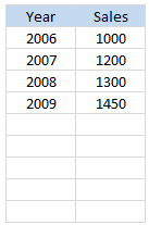 In our case the data should be filled in the following table. As user keeps on adding new rows we will have to update our chart’s source data.
Lets assume the data table is in the cell range: $F$6: $G$14
2. Write OFFSET formulas and create named ranges from them
Ok, the problem is that as and when we add a row at the end (or remove a row), we should update the chart’s data range. For this, we can use OFFSET formula.
A refresher on how to use OFFSET formula:

3. Create a new named range and type OFFSET formula
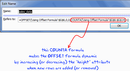
Create a new named range and in the “refers to:” input box, type the OFFSET formula that would generate a dynamic range of values based on no. of sales values typed in the column G. I have used the below formula. You can write your own or use the same technique.
=OFFSET($G$6,0,0,COUNTA($G$6:$G$14),1)
Set the named range’s name as “sales_data” or something like that.
Now repeat the same for years column as well and call it “years_data”
4. Create a column chart and set the source data to these named ranges
Create a column chart. For the source data use the named ranges we have just created.
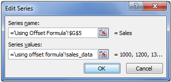
Important: You must use the named range along with worksheet name, otherwise excel wont accept the named range for chart source data.
That is all, now your chart is dynamic
Download the Dynamic Chart Ranges Tutorial Workbook
Click here to download the dynamic chart ranges workbook and use it to learn this trick. I have given Excel 2007 file since the file includes tables.
Bonus Tip: Edit chart series data ranges using mouse
If you have no time for writing lengthy formulas or setting up data tables, you can still save time when editing chart series data ranges. Just select the series by clicking on the chart. Now excel shows highlighted border around the cells from which the chart series is created. Just click on the bottom-right corner and drag it up and down to edit the chart series data ranges. (more: Edit formula ranges using mouse)
See the demo to understand this:

More tricks to make dynamic charts using Excel
Here is a list of tutorials and examples recommend just for you. Go check them out and make your charts even more dynamic.
- Filter Charts just like you filter Data
- Select and show one chart from many
- Dynamically Group Related Data in the Charts
- Use Data Filters as Chart Filters and Make Dynamic Charts
- A Dynamic Donut Bar Chart – Show total and break-ups in an interesting way
Tell me about your experience with dynamic charts using comments.


12 Responses to “29 Excel Formula Tips for all Occasions [and proof that PHD readers truly rock]”
Some great contributions here.
Gotta love the Friday 13th formula 😀
Great tips from you all! Thanks a lot for sharing! bsamson, particularly you helped me on a terribly annoying task. 🙂
(BTW, Chandoo, it's not exactly "Find if a range is normally distributed" what my suggestion does. It checks if two proportions are statistically different. I probably gave you a bad explanation on twitter, but it'd be probably better if you fix it here... 🙂 )
Great compilation Chandoo
For the "Clean your text before you lookup"
=VLOOKUP(CLEAN(TRIM(E20)),F5:G18,2,0)
I would like to share a method to convert a number-stored-as-text before you lookup:
=VLOOKUP(E20+0,F5:G18,2,0)
@Peder, yeah, I loved that formula
@Aires: Sorry, I misunderstood your formula. Corrected the heading now.
@John.. that is a cool tip.
Hey Chandoo,
That p-value formula is really great for a statistics person like me.
What a p-value essentially is, is the probability that the results obtained from a statistical test aren't valid. So for example, if my p value is .05, there's a 5% probability that my results are wrong.
You can play with this if you install the Data Analysis Toolpak (which will perform some statistical tests for you AND provide the P Value.)
Let's say for example I've got two weeks of data (separated into columns) with the number of hours worked per day. I want to find out if the total number of hours I worked in week two were really all the different than week one.
Week1 Week2
10 11
12 9
9 10
7 8
5 8
Go to Data > Data Analysis > T-Test Assuming Unequal Variances > OK
In the Variable 1 Box, select the range of data for week 1.
In the Variable 2 Box, select the range of data for week 2.
Check "Labels"
In the Alpha box, select a value (in percentage terms) for how tolerant you are of error.
.05 is the general standard; that is to say I am willing to accept a 95% level of confidence that my result is accuarate.
Select a range output.
Excel calculates a number of results: Average (mean) for each week's data, etc.
You'll notice however that there are two P Values; one-tail and two-tail. (one tail tests are for > or .05), the number of hours I worked in week two is statistically equivalent to the number of hours I worked in week one.
So here’s a way you might want to use this. You put up a new entry on your blog. You think it’s the best entry ever! So you pull your webstats for this week and compare it to last week. You gather data for each week on the length of time a visitor spends on your website. The question you’re trying to prove statistically is whether there’s an average increase in the amount of time spent on your website this week as compared to last week (as a result of your fancy new blog post). You can run the same statistical test I illustrated above to find out. Incidentally, it matters very little to the stat test whether the quantity of visitors differs or not.
Anyhow, the Data Analysis toolpack doesn't perform a lot of stat tests that folks like me would like to have access to. In those cases I have to either use different software, or write some very complicated mathematical formulas. Having this p-value formula makes my life a LOT easier!
Thanks!
Eric~
Fantastic stuf..One line explanation is cool.
Thanks to all the contributors
OS
Take FirstName, MI, LastName in access (you can fix it to work in excel) capitalize first letter of each and lowercase the rest and add ". " if MI exists then same for last name:
Full Name: Format(Left([FirstName],1),">") & Format(Right([FirstName]),Len([FirstName])-1),"") & ". ","") & Format(Left([LastName],1),">") & Format(Right([LastName],Len([LastName])-1),"<")
I teach excel, access, etc etc for a living and i have my access students build this formula one step at a time from the inside out to show how formulas can be made even if it looks complicated. Yes I know I could just do IsNull([MI]) and reverse the order in the Iif() function but the point here is to nest as many functions as possible one by one (also I illustrate how it will fail without the Not() as it is)
Extract the month from a date
The easiest formula for this is =MONTH(a1)
It will return a 1 for January, 2 for February etc.
if in a column we write the value of total person for eg. 10 if we spent 1.33 paise each person then how we get total amount in next column and the result will in round form plzzzzz solve my problem sir................... thank u
@Anjali
If the value 10 is in B2 and 1.33 paise is in C2 the formula in D2 could be =B2*C2
If the values are a column of values you can copy the formula down by copy/paste or drag the small black handle at the bottom right corner of cell D2
kindly share with me new forumulas.
How to convert a figure like 870.70 into 870 but 871.70 into 880 using excel formula ? Please help.