
Bar & Column charts are very useful for comparison. Here is a little trick that can enhance them even more.
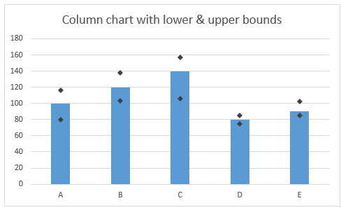
Lets say you are looking at sales of various products in a column chart. And you want to know how sales of a given product compare with a lower bound (last year sales) and an upper bound (competition benchmark). By adding these boundary markers, your chart instantly becomes even more meaningful.
How to create a chart with lower & upper bounds?
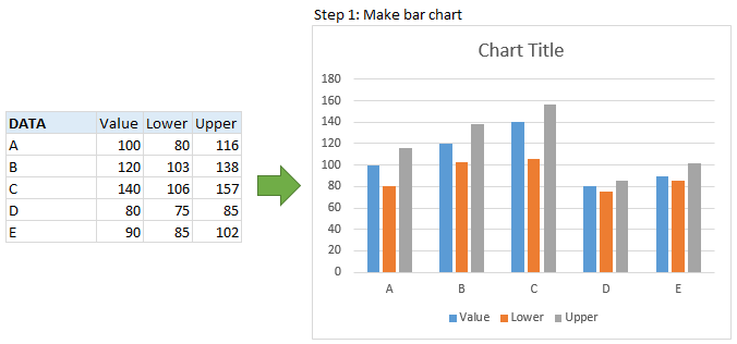
1. Select data and make a column chart
Lets say your data looks like this. Select it all and insert a column chart from insert ribbon.
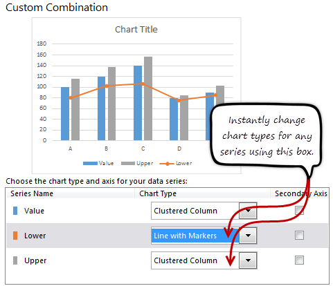
2. Convert lower & upper columns to lines
 In Excel 2013:
- Right click on either lower or upper bound columns.
- Choose “Change series chart type…”
- Select “line chart with markers” as the chart type for both lower & upper series
- Done!
In earlier versions:
- Right click on lower series
- Choose “Change series chart type…”
- Select “line chart with markers”
- Repeat the process for upper series
- Done
- Related: How to create combination charts in Excel?
After this step, your chart looks like this:

3. Set line color to “no line” and format markers
This is easy. Just set the line color to “no line” and format the markers so that they are prominent.

Your column chart with lower & upper bounds is ready.
Bonus step: Custom shapes for lower & upper bounds
If you want something fancy, you can use custom shapes for lower & upper bounds, as shown below.

To get this:
- Draw custom shapes using drawing tools in Insert ribbon.
- Make sure they are really small (else the markers will be shown at wrong places)
- Copy the shape (CTRL+C)
- Select marker series for which you want this shape.
- Paste (CTRL+V)
- Done!!!
Video tutorial of Column chart with lower & upper bounds
Here is a video tutorial of column chart with lower & upper bounds.
This video is also part of my Excel School program. If you like the video, you are going to love our Excel School program, where more than 50 such videos will help you become awesome in Excel.
Click here to know more about Excel School & join us.
Download the chart workbook
Click here to download the workbook. It contains column chart with lower & upper bounds example, detailed instructions and custom shape example.
When do you use lower, upper bounds in your charts?
I use this technique all the time. I apply markers for extra data like average, KPI targets, last year values etc. Here is one more example.
What about you? Do you use lower, upper bounds in your charts? In which scenarios you apply them? Please share your experiences using comments.
For more charting tips…
Make sure you check out our charting page. It has 100s of Excel tutorials, templates & design examples on charts.
If you still want more, consider joining Excel School. You will be a charting pro soon.


20 Responses to “Untrimmable Spaces – Excel Formula”
Hi Chandoo,
First of all, HAPPY NEW YEAR!!! Wish you and your family another fruitful year ahead.
To answer your question: Power Query is the best way to trim. 🙂
Btw, if Power Query is not available, then formula would absolutely do... but did you forget to mention also Char 32?
One more question: Is the trailing minus meant to be a negative number? Maybe only the sender knows... 🙂
Cheers,
I just see your PQ way, it is amazing, I think it is the most simple way.
No idea how it did it?
I know these spaces can be a real pain but these days I advise Excel users to learn and use Flash Fill and that will learn what to do pretty quickly.
Highlight range to be cleaned. Then, in Replace, hold down the Alt key and type 0160. Replace with nothing.
I accomplished this by writing a macro to go through all the possible unprintable characters. Looped through the range.
@Steve
Brute force works just as well, its just slower
I use a different method here. First, I will copy the data from Excel and paste it in a notepad. In Notepad, I will do a Find Blanks (Space " ") and Replace (Empty) with nothing.
Then you can copy the data from Notepad and paste it back to Excel which will be a perfect number as you desire.
But Thanks for the formula. Its probably the 2nd out of 8 tricks as Chandoo mentioned. Waiting for the rest among 8 from other users 🙂
Hi....
You don't always need notepad for that. I use the Find/Replace is Excel works just fine.
I don't understand the x's. Why weren't they removed in the formula? Or are they part of some sort of numeric formatting that I'm not familiar with? I saw how you handled the non-breaking spaces and the dashes, but am confused about what role the x's played in all this.
Thanks!
Hi Andrew ,
The xs have been used solely to demarcate the actual data text ; thus , without the x in place at the end of text , as in :
x 4,124,500.00 x
it would be impossible to know that there are unwanted trailing characters , in this case , after the last 0.
These xs are not part of the original data text , nor are they used in the formulae ; they are put in only so that readers can visualize the individual items of data as they are in practice. Think of them as imaginary delimiters.
Oh, that makes sense! Thank you for the explanation. I had a feeling it was something along those lines.
You can type this character using the Keys Alt+0160.
Very useful to replace this Character using Find and Select resource.
For many years, my jobs have included ETL tasks and I built this macro to help long, long ago. I tweak it every now and again. Many co-workers, past and present, have it wired to a button on their toolbar.
Sub Clean_and_Trim()
'CAUTION: Strips leading zeroes -- do not use on zipcodes, etc.
If Application.Calculation = xlCalculationAutomatic Then
Application.Calculation = xlCalculationManual
Revert = 1
ElseIf Application.Calculation = xlCalculationManual Then
Revert = 0
End If
For Each Cell In Selection
For x = Len(Cell.Value) To 1 Step -1
If Asc(Mid(Cell.Value, x, 1)) = 160 Then
Cell.Replace What:=Chr(160), Replacement:=" ", LookAt:=xlPart, MatchCase:=True
End If
If Asc(Mid(Cell.Value, x, 1)) = 32 Then
Cell.Replace What:=Chr(32), Replacement:=" ", LookAt:=xlPart, MatchCase:=True
End If
Next x
If Cell.Value "" Then
Cell.Value = Application.Clean(Application.Trim(Cell.Value))
End If
Next
If Revert = 1 Then
Application.Calculation = xlCalculationAutomatic
ElseIf Revert = 0 Then
Application.Calculation = xlCalculationManual
End If
End Sub
This is awesome! What if you have several characters you need to have removed? What would be the easiest way as I can imagine there are several ways.?
# - 35
$ - 36
- 62
/ - 47
, - 44
. - 46
" - 34
: - 58
This is typical case of a Fitbit data export to Csv file. Each number has CHAR160 as thousand separator.. how smart Fitbit, thank you 😉
By the way, i prefer to copy the character, and use find and replace.
Sometimes it happens if you copy a table from outlook and paste it in excel. When you apply formula on those cells you will get error. What i use to do is
copy one character that looks like space,
select the entire range,
go to Find and replace,
Paste the copied character in Find option
Leave the replace option unfilled..
click on replace all..
All the errors shall be converted in to proper values..
Process looks lengthier.. but it is one of the simplest method
If Clean, Trim, and Substitute, or Find and Replace does not complete the job, I usually enter a value of 1 in an empty cell. Copy the Value of 1, Highlight the range of text numbers, and Paste Special, Values, Multiply. This site is great!
You can use Dose for Excel Add-In that can quickly clean huge data with one click besides more than +100 new functions and features to add to your Excel to save time and effort.
https://www.zbrainsoft.com
Hi,
I have a problem in excel. The sheet attached herewith.
TABLE CONFIG 2/6
A B C D E F G H
1 WEIGHT1 43,599 WEIGH2 62500 WEIGHT3 77000 WEIGHT4 66,500
2 DEDUCTION1 15,000 DEDUCTION1 15,000 TEMP 0 DEDUCTION2 11,005
3 RESULT 58,599 RESULT-1 77,500 RESULT-2 77,000 RESULT-3 77,505
4 RESULT SUBSTRACT 0 0 0
5 REQUIRED VALUE 77,500 77,000 77,505
Note: 1- RESULT (58599) IS TO BE DEDUCTION EITHER FROM D4 OR F4 OR H4 WHICHEVER IS MOST
LEAST CELL AMONG RESULT-1 OR RESULT-2 OR RESULT 3.
2-HENCE, RESULT VALUE $B$3 IS TO BE PRESENTED ON CELL EITHER D4 OR F4 OR H4 WHICHER IS
MOST LEAST VALUE
3-FORMULA =IF(E8<H8,$B$9,IF(E8<J8,$B$9,IF(H8<J8,$B$9,IF(H8<E8,$B$9,IF(J8<H8,$B$9))))))
CREATED ON CELL D4,F4 & H4 DID NOT WORK.
PLS FOR YOUR HELP.
THANK YOU
@R
Why not ask the question in the Chandoo.org Forums
https://chandoo.org/forum/
You can attach a file there