
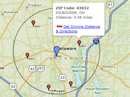
Recently, I had a peculiar problem. I have a list of zip codes and I wanted to find out nearest zip codes for each of them.
Now, If I wanted to find out near by zip codes for one area, I could go and search in Google. But, how to do it for dozens of them?
Today, lets understand how you can use Excel (that’s right) to do this automatically. We will be using Excel 2013 for this.
A little background – Excel 2013 Web Formulas
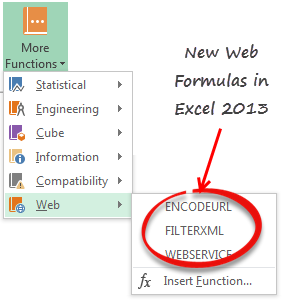
In Excel 2013, Microsoft has introduced 3 powerful new formulas. These will help you fetch & parse XML / HTML data from web. The formulas are,
- ENCODEURL: to encode web URLs (replaces special characters in URLs with % codes like space becomes %20, / becomes %2F etc…)
- WEBSERVICE: connects to a webservice / website and fetches response as XML / HTML.
- FILTERXML: extracts a portion of XML/HTML using specified XPATH.
Using these formulas and web services, we can quickly fetch near by zipcodes for any input value.
Step 1: Find a web-service that can tell us near by zipcodes
I am sure there are many web sites that can offer a service like this. After searching a while, I came across a website called as geonames.org which has many webservices around address / zip code search. The service I have used is,
This service is available as XML & JSON. Since Excel 2013 formulas only process XML data, I went with XML service. The service API url is this:
http://api.geonames.org/findNearbyPostalCodes?postalcode=ZIPCODE&country=US&radius=15&username=UNAME&maxRows=10
ZIPCODE is where you enter the zipcode from which you want to find nearby zipcodes
UNAME is where you enter your user name for geonames.org. Click here to register with geonames.org.
Step 2: List all original Zip codes in a column
This is simple. Just paste all original zip codes in a column.
Step 3: Write WEBSERVICE Formula
First enter the API URL in a cell like B1. (Make sure your user name is included in the service url)
Now write WEBSERVICE formulas so that we can fetch XML listing for each of the zip codes. Assuming zip codes are in A3:Ax, in adjacent column write =WEBSERVICE(SUBSTITUTE($B$1,”ZIPCODE”,A3))
And drag it down to fill down the formula for all zipcodes.
Step 4: Write FILTERXML formulas
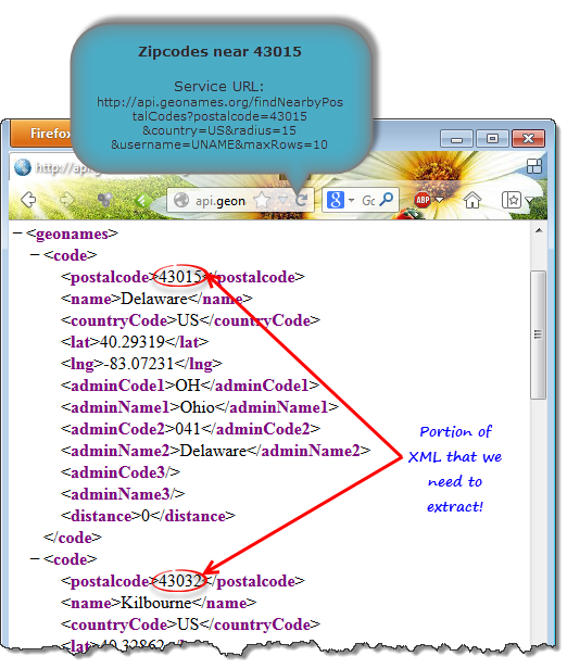
Now that we have full XML corresponding to each zip code, we need to parse this XML to extract the nearby zip code numbers. The original XML looks something like this:
To extract the zipcodes alone, we need to use FILTERXML formula.
FILTERXML takes 2 inputs – XML text, Xpath.
XML text is what WEBSERVICE has generated.
XPATH will tell Excel, which portion of XML to extract.
What is XPATH?
If you imagine XML as a tree, then XPATH is the language you use to tell how to navigate to a certain node in that tree. Since XPATH is a complex world, I think explaining all the syntax & nuances can be hard. So I will leave you with 2 useful links.
So what is the XPATH for nearby zip code.
As you can see in above image, the response from geonames has 10 code nodes, each containing one zip code (in the postalcode child node).
If we write =FILTERXML(b3,”/geonames/code/postalcode”) we will get all the postalcodes as an array.
Since Excel cannot show arrays in cells, it will show one of the 10 values.
So we need 10 cells to show these 10 zip codes. Once you have 10 cells, you can use either INDEX formula or alternative XPATH syntax (/geonames/code[1]/postalcode for first code, ../code[2]/.. for second code etc.) to extract all the 10 zip codes.
Things to keep in mind
Web formulas (WEBSERVICE formula to be specific) can be really slow depending on your net connection and webserver speeds. Since for most data, we do not need a live connection once the data is fetched, it would be good idea to replace WEBSERVICE formula with results once you have the XML.
Also, working with XPATH can be frustrating if the source XML is not correctly formatted or you are not familiar with right XPATH commands. In such cases, use SUBSTITUE or Text formulas to strip away un-necessary portions of webservice text before feeding it to FILTERXML.
Last but not least, Web formulas are compatible only with Excel 2013 or above. So you need to replace all formulas with results when emailing the workbooks to colleagues who are using older versions of Excel.
Download Example File – Finding Nearby Zipcodes
Click here to download the Excel workbook. Play with it to understand how the formulas are working. Please note that this file is protected as I do not want you to use my username for geonames.org.
Do you use Excel Web formulas?
Although Excel 2013 includes only 3 web formulas, they can let us do several interesting things. I am playing with them often to see what additional uses we can put them to.
What about you? Have you used Excel 2013 web formulas? What is your experience like? Please share using comments.
More on using Excel to get data from web
If you often need data from external websites for your Excel analysis work, check out below articles too:


20 Responses
This can also be done in Excel 2010or does it work only for 2013?
To do it in prior versions you must use VBA.
ok thanks for the info…
All by itself, a downlevel version of Excel doesn’t support the new functions introduced in Excel 2013. However, using the Excel PowerUp add-in from officepowerups.com (http://officepowerups.com/downloads/excel-powerups-premium-suite/) you can extend Excel 2010, 2007, and 2003 to have the functions as well, without installing Excel 2013. And as a bonus, the Excel PowerUp version of WEBSERICE supports POST as well as GET.
Great tip Chandoo !!
Thank you
Great Idea! And thanks for explaining it so nicely. 🙂
I just wanted to know can i use this function to access password protected web-services? I mean is there any way I can pass the web-services credentials to this function.
Thank you chandoo! Please if you do not complicate, help me to build the Xpath for this XML. I want to get value tag.
My path is “/ValCurs/Valute/Value”, but unfortunately it does’t work.
Very cool. This is also not far from where I grew up!
Havent started using excel 2013, but this formula seems can be very handy.
is this tutorial this valid? Have been trying to do it with no joy. tks
Using web formulas in Google Spreadsheets to monitor product prices in Amazon [Guest post on Labnol.org]
http://www.labnol.org/internet/monitor-web-pages-changes-with-google-docs/4536/
Chandoo
Just want to make you aware – by using the evaluate formula in Excel 2013 and stepping into the function(s) one can actually see your username etc.
Could anyone point me in the right direction of doing something similar in excel 2003 (most likely with VBA) and using UK post codes?
Just so you know, nearest postal codes doesn’t work in Canada. I have tried some Montreal codes (H2T, H1A) and it gives back only a few answers as if radius was always set to a low value (always less than 5).
Proof that I should have a lot of answers:
http://www.findthepostalcode.com/location.php?province=QC&location=Montreal
Forget my last comment… MaxRows=5…
Thanks for nice tutorial.. can you please do example for Json since more sites are offered based on Json.Thanks
Does anyone know if there is a formula to pull back historical exchange rates? I need to convert financials for a company into various currencies from my base currency at the conversion rate for the month selected. So for example my USD value pulled through for December 2010 is $4500 but I want to convert it into GBP using the exchange rate at the time.
@Jose
Not really sure about the relevence of this post to Excel
I use http://www.xe.com
then goto Tools, Current and Historical Rate Tables