


Update: As of Sept 3rd, 2010, this code or approach no longer works. Twitter has taken themselves too seriously to disable a working protocol in lieu of complicated oAuth. I am keeping the post intact for amusement and knowledge of xmlhttp works.
Twitter is fun. You can stay in touch with your friends and followers, 140 characters at a time.
Out of curiosity I opened the twitter api documentation today to see if it is possible to build an excel based desktop client to post messages to twitter.
It turns out that, doing this using twitter api is relatively simple. So I went ahead and built an excel sheet using which you can post messages to your twitter account. Interested? Read on
Create a new MS Excel file and make a data entry form like this
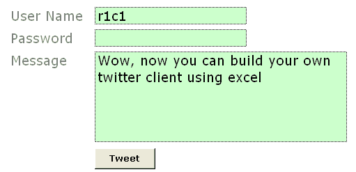
You can insert the button using form controls. Go to menu > view > toolbars and select “forms”.
Now select the button control and draw it on your sheet.
Excel will show a dailog asking which macro to run when that button is pressed. Enter the name as “tweetThis” or something cool.
Make sure you adjust the text color of password field same as background. That way your colleague (say hello to her from PHD) cannot look over your shoulder and know your twitter password.
PS: if you are using Excel 2007, form controls will be available in “Developer” tab of ribbon. If you don’t see developer tab, you must turn it on from “excel options”. Press office button and select excel options. I guess the option will be in “Advanced” area.
Create named ranges for your data
(this step is not mandatory)
We need just 3 fields of data to post a message to your twitter account. User name, Password and Message . Select each of the 3 cells and create named ranges for them. Name them something meaningful like “tusername”, “tpasswd” and “tmessage”. To create a name for selected cell, just press menu > insert > name > define (press the create name button in excel 2007)
Now, the fun part, writing macro code to post your message to twitter
The actual code is no geek stuff. We will use XMLHTTP object to do our work.
What is xmlhttp? it is the same object your browser uses to dynamically receive and send data from websites. It is the stuff behind all those cool AJAX powered sites.
First, right click on the “tweet” button you have created and select assign macro option. In the window it would show your macroname (tweetThis). Select it and click on edit button. This will open VBA Editor. Don’t freak out. 🙂
Our code needs to do the following stuff:
- Create an xmlhttp object
- Use twitter API’s post method and post the message
- Get the status and display it in debug window (just so that we would know if something went wrong)
- Close the xmlhttp object
I have written the below code, but I am sure you can write your own looking at how simple it is.
Sub tweetThis() Dim xml, tUsername, tPassword, tStatus, tResult Set xml = CreateObject("MSXML2.XMLHTTP") 'get the username entered by you in named range tusername tUsername = Range("tusername") 'get the password entered by you innamed rangetpasswd tPassword = Range("tpasswd") 'get the message entered by you innamed range tmessage tStatus = Range("tmessage")xml.Open "POST", "http://" & tUsername & ":" & tPassword & "@twitter.com/statuses/update.xml?status=" & tStatus, False xml.setRequestHeader "Content-Type", "content=text/html; charset=iso-8859-1" xml.Send tResult = xml.responsetext 'you can view Twitter’s response in debug window Debug.Print tResult Set xml = Nothing End Sub
Finally, enter your user name and password and a test message and test your code
If everything is fine, you should be able to tweet from that spreadsheet. Here is a sample message if you don’t know what to tweet:
Wow, http://chandoo.org/wp just posted a cool new way to make your own twitter client
You can easily extend this code to check someones status message, DM or message someone or analyze twitter stream. For processing twitter data you can use DOM parser objects from VBA.
Download Twitter from Excel Application and Play around with the code
Go ahead and download the twitter from excel app and learn by opening the code etc.
That is all. Do you like this ?
Cool, then please Tweet About This!, add this to your delicious bookmarks, stumble this page.
If you are new to PHD, I encourage you to sign up for our e-mail updates or add this blog to your reading list because we post cool and fun excel and charting stuff almost every weekday.
Check out other cool excel and spreadsheet stuff
Track your investments using Excel
Build an expense tracker using google docs
Make your own Amazon Deal Tracker in Excel
Findout when that iPod is available for cheap. Learn xpath and track almost everything


94 Responses
How about a UI version?
Although I signed up for Twitter a while ago and linked my Twitter account to Facebook so that my status would be in sync, I’ve never found a way of sending tweets that is convenient enough for me to do more than just the occasional update.
Thanks to your post, I now have a commandbar button with a neat Twitter logo that loads a userform that allows me to tweet from the application I spend about 9 hours a day staring at – no visiting a site specifically to tweet, running a separate app or dealing with an annoying mobile interface.
If this doesn’t allow me to get more into Twitter then I guess nothing will!
Awesome, Will check it 🙂 Thanks for sharing
Good one dude.
Will try.
-Nikhil
Bit obvious this really, but I found you have to do a replace on any character in your tweet that can get mixed up in the XML, e.g. “&”.
Replacing these characters with their hex encoded equivalents allows the tweet to go through.
@JP.. you mean an add-in.. well, I wanted to explore xmlhttp and this is my first time. So I tried to keep it simple, but adding a ui or userform is straight forward and simple
@Gordon: neat stuff… may be you can share this with us so that JP can download and play with it :), btw, you could use some version of urlencode () to achieve clean up the message content. I didn’t explore all that, but a very good suggestion.
@Kunal: welcome to PHD and thanks.
@Nikhil: thanks dude…
This was awesome. Thanks.
One more thing, I’m not a fan of Twitter at all, but isn’t there some kind of limit to the number of words or characters you can post at one time? If so, you might want to add a check that makes sure Range(“tmessage”) isn’t too long.
HTH
@curtisincalgary: thank you 🙂
JP: the download has a character count to keep the message to 140 chars. Also twitter api is smart enough to take just 140 chars if you are sending messages. so there is little to worry.
Here it is Chandoo, the UI version of your Twitter code I’ve been working on:
http://www.codeforexcelandoutlook.com/blog/2009/02/excel-to-twitter/
Take care,
JP
Wauw, tnx for sharing. I am going to try this one! :p
Question: Can we tweak this app so that it can archive the tweets??
@Brijesh: yes, yes we can. Twitter sends the response back in xml format. use the DOM object to chomp the xml to what you want and you have a tweet-archiver-spreadsheet ready.
Thanks. I guess, that is something for weekend.
Taking this a step further: How can I archive the tweets of few people whose ideas I really look forward to? Can this be achieved using DOM?
@Brijesh: yeah, DOM is just a framework to parse the XML (or other data that follows the document object model, like web pages etc). If you are looking for a tweet archiver for your fav people (or #topics), here is how you can do it,
First follow the fav people
now ask excel to go to your following page and capture all updates
parse the updates using dom and place them in a table on the spreadsheet
repeat often
One of my planned updates for Post To Twitter is to allow you to read others’ tweets. I say “planned” because I’m trying to figure out how to read the XML response, turn it into an XML document, and then parse that. That, and a lot of candle lighting and praying.
@JP: and coffee too 🙂
on a serious note, I found twitter api to be much more easier to work with than some other stuff out there. Also, one more way to work around the parsing problem could be to pass the xml through some services that spit out csv / txt (like yahoo pipes, which incidentally has the ability to take dynamic xml / rss urls as input and runs them on the pipe to return the output in the format your prefer, like JSON)
Hi,
You know what I would really really like (apart from archiving) is to Schedule the tweets. That I guess, is relatively easier and would be fabulous.
@brijeshj
Yeah – this would be awesome if someone can figure out a way to schedule the Tweets based on data already in an excel spreadsheet.
I work for a cable network and we are just starting to use Twitter to give program updates to our fans. Every week I get the program guide with show name, time, episode description and I would add a shortened link field to this for the show page. If I could have tweets scheduled 30 minutes before the show airs that would be epic.
If anyone wants to experiment with trying this please e-mail me: mr dot escandon at gmail dot com
@Paul
Getting a list of users to send a message to from a range in Excel is not a problem, the issue is that Twitter has a limits on both the minimum time between tweets (5 minutes I think) and maximum tweets per hour (140?), making Twitter all but unusable for a notification service like you are proposing.
Hi Chandoo,
I’m also trying to develop a vba form where getting some values to enter into the spreadsheet. The point is I’ve got to recover a value from an entryfield ( with no format. I don’t know how formatting textfilelds in vba forms ) and set the value of the cell in the spreadsheet.
The decimal character is ‘,’. When I do not enter decimals, the value is captured OK, but when I enter decimals, the cell loses its format.
Do you know how can I format the value of the entryfield ?
Thanks for your excellent blog.
I downloaded the .xls file and tried it. I get this mashed up Windows Live content stuff. What does that mean?
@Tudza: I think you have downloaded the file by right clicking on the url. You need to actually visit the url and download the excel from there. Let me know if you face some difficulty….
Similarly, I developed a full-featured twitter client on Excel called “TweetSheet”. You can take a look!
http://iphone-chieftain.blogspot.com/2009/04/tweetsheet-10-released.html
@Alex.. awesome stuff… Thanks for sharing this with us.
thats great that you are talking about the twitter api,a good example of searching with the twitter api is on twiogle.com because you can search on twitter and google at the same time.
I have tried sending messages through Excel and it works great. I also wrote some code to schedule messages and all works like a charm. It seems Twitter has problems with %-sign. If I send a message with the %, ir goe swrong and doesnt want to go. Do you know how to solve this?
Thanks
Make sure that you have set the correct content-type as below:
xml.setRequestHeader “Content-Type”, “application/x-www-form-urlencoded”
@Eddy: it could be because % is a special character in webforms. As suggested by Alex, you can try changing the encoding type.
Excel-lent post! Thanks.
I figured out the % problem, which has to do with the way XML handles the message. If you add 25, the message will be correct in Twitter. So %25 on the Excel sheet looks like % in Twitter.
I figured out the % problem, which is caused by the way the XML message is handled. If you use %25 in your Excel message, it will look like % in Twitter.
Hi! I downloaded tweetsheet and am getting a runtime error 800c0005 (after press tweet button, of course) while using excel 2007 on vista… any ideas? Thanks in advance!
What is Twitter and How Can I Use It?
@Craig… sorry, I didnt see your comment earlier. Is the problem resolved? May be the firewall or proxy server is preventing you to access twitter… ? This error occurs when firewalls block the msxml object which we are using in this excel file.
@Cinocefalo… Twitter is next god.. :P, I am kidding, it is just another social media tool that you can use to say what you are upto in less than 140 chars at a time… try it, you might find a cool use for it.
Your wonderful idea but running into some problems. The update fails and I get a debug at xml.send
xml.Open “POST”, “http://” & tUsername & “:” & tPassword & “@twitter.com/statuses/update.xml?status=” & tStatus, False
xml.setRequestHeader “Content-Type”, “content=text/html; charset=iso-8859-1”
>>>>xml.Send
@Lanier… the most likely scenario for this error is when your firewall blocks outgoing communications from xmlhttp object. I had the same problem when I tried this from office comp (where twitter is blocked). But when I try it from home, it worked perfectly. Can you try this in some other comp and let me know if the error persists.
Chandoo,
Still the same problem or home network or company. I download another excel that works fine for home and company network. TweetSheet2.0.1.xls is the name of the excel sheet that works. But is much more complicated
I use the following module to send tweets in Excel in TweetSheet.
Sub tweetMessage(sStatus As String, sReplyId As String, sTwitterID As String, sTwitterPwd As String)
Dim xml As Msxml2.XMLHTTP
Dim sXMLMsg As String
Set xml = New Msxml2.XMLHTTP
If Len(sReplyId) > 0 Then
sXMLMsg = “in_reply_to_status_id=” & Trim(sReplyId) & “&status=” & sStatus
Else
sXMLMsg = “status=” & sStatus
End If
xml.Open “POST”, “http://@twitter.com/statuses/update.xml”, False, sTwitterID, sTwitterPwd
xml.setRequestHeader “Content-Type”, “application/x-www-form-urlencoded”
Call xml.send(sXMLMsg)
Set xml = Nothing
End Sub
When I hit the tweet button I get an error message. “Compile error: Syntax error” The macro formula is brought up behind the error and debug program is behind that. How do I fix this Please help.
@Steven… Have you copy pasted the code from above? May be it is the dirty quotes or something. Can you try it from the downloadable workbook?
I tried pasting the macro above, now I get an error msg stating it may not be available. Now the tweetthis is gne and I cantget it back.
Alex ,
I am getting arugment not optional with your code. Sorry for being dense. But how do you program the excel sheet to accecpt your vaules.
Chandoo,
Still no luck with you code.
Lanier
@Steven: You might have pasted same sub twice. Can you close the workbook and try to work with the downloadable workbook. The link is in the post.
@Lanier: Over the last few days, twitter has been going through tremendous amounts of downtime. May be that is why the code is bouncing…. ?
Just pass the empty string “” to the optional argument, such as sReplyId.
Chandoo,
No luck. Still the same. Crashes at xml.send
Anyone know if this can be done using an oauth token instead of relying on inputting a password?
Is it possible to make this work using Excel 2003? Thanks!
@Rolan.. this script works in Excel 2003 as well. Are you facing any problems?
I haven’t made it worked in Excel 2003 yet, but I was able to make a prototype in MS Access 2007 which opens the possibility of creating a database of tweets to be posted according to a pre-determined time.
I like your articles Chandoo. I just wana asked if its ok for you to provide a link to my site http://www.mymsoffice.net and I will also link to your site. Thanks!
@Rolan.. that is a cool idea, using db and timing the tweets.
btw, coming to your request, I do not link to other sites on my blog just like that. I provide links to useful excel, charting and story-telling articles from time to time on posts. I like the content on mymsoffice.net and have subscribed to it on my reader. I will share interesting articles to my readers through that and may be in an upcoming “excel links” post.
That was so cool. You know how it says “less than 5 seconds ago from API”? Is there a way to make the “API” part read “Excel”?
@sean
No, you need to get a developer API key to have your application’s name appears here. This is a process that requires you to submit your application for testing by Twitter.
This is very inusual, something i didn’t expected from excel and so cool. I’ve been vb programer for a year and i didn’t know that u can make XMLHTTPRequest objects from it. I’m gonna try when i have the chance. This makes me think that my web page is not that cool anymore thanks to you
chepe263
Quitter Admin.
Wow, simply the best way to tweet! Just downloaded your file and learning to modify the codes to use privately….
if you have developed variations please let us know,
thanks
Was quite excited about this but this seems to suggest I won’t have much luck from work…
407 Proxy Authentication Required
Proxy Authentication Required
Unable to complete request:
Access denied due to authentication failure.
To complement this cool macro, I wrote a function for fetching tweets, so now you don’t need to visit Twitter at all 🙂
http://mikaelspage.blogspot.com/2010/05/fetching-tweets-to-excelwordppt.html
Until it has OAuth support, for those wanting to use this code after June 2010, it should be easy to modifiy it to use http://www.supertweet.net/api
Fantastic !! Awesome !! Thank you very much for sharing.
Does anyone have updated code with use of OAuth?
@LK… nah.. But twitter is still supporting REST API. I tried to look at the oAuth API, but it seemed like too much hassle for a fun project like this. Nevertheless, I would be curious to know if anyone implemented it in vba.
@Chandoo No more basic authentication for Twitter. You have no choice but use OAuth. I think the hassle is inevitable now. Any ideas?
Chandoo:
I found your code a year ago and used for real-time football game updates all fall while keeping stats for a high school football team. It worked really well. I am preparing for another football season, first game tomorrow, and testing my setup. Last Monday the tweetThis code worked just fine. Today it does not. Did Twitter change something that I need to adjust the code for?
Thanks, JLS
The macro was working fine until yestarday. But today it seems twitter.com has changed something and this macro is NOT working anymore…. Which is too sad. How can we work around?
@all.. I am sorry, but the code no longer works. Twitter has taken a bold step of disabling RESTful API and chosen to use oAuth. Don’t ask me why. I guess they didnt want to care about all those developers who wrote code using earlier authorization mechanism.
Please note that I am learning about oAuth and I may post an updated macro sometime in future. Meanwhile, if you cracked the oauth nut, please share your insights / code using comments.
You should try using an OAuth gateway, like Simple Auth Twitter (http://simpleauthtwitter.heroku.com/) or SuperTweet (http://www.supertweet.net/).
Personally, my client of choice until the change was TweetSheet (http://iphone-chieftain.blogspot.com), but it seems like the macros in there are password-protected 🙁
Go to http://simpleauthtwitter.heroku.com and request a authorization key and insert it on the following code:
Sub tweetThis()
Dim xml, tStatus, tResult
Set xml = CreateObject(“MSXML2.XMLHTTP”)
‘get the message entered by you in named range tmessage
tStatus = Range(“tmessage”)
xml.Open “POST”, “http://simpleauthtwitter.heroku.com/tweet?api_key=YOURKEY&status=your-messageSimple”
& tStatus, False
xml.setRequestHeader “Content-Type”, “content=text/html; charset=iso-8859-1”
xml.Send
tResult = xml.responsetext ‘you can view Twitter’s response in debug window
Debug.Print tResult
Set xml = Nothing
End Sub
Best regards,
Marcelo Araujo
Congratulations and thank you, Marcelo.
It is working fine. And thank you for sharing.
Yea – no to simpleauthtwitter. I do not pass my userid/password/api keys, etc through any gateway. If it cant be written in pure code that stays on my box then I wont use it. Has anyone found a way to write pure code, without the use of someone else’s library (a black box that I do not trust) where the control of the code is in the hands of us, the developers?
I tried your code Marcelo, and I don’t get anything to show up in my twitter feed. any ideas? I am using 2003 btw.
Wow this is cool dude. Hey I have a tough task of having to visit twitter daily and import daily trends into excel and track them for my boss. Is this something that you can do for me like the excel tool that automatically gets the daily, weekly or monthly trends into excel. So i dont have to manually do the work.
Heres a vba.rest library, including a twitter entry.
http://ramblings.mcpher.com/Home/excelquirks/json/rest
Direct import to excel of the fields you need with no coding required.
Bruce.
Hi, is this code compatible with the new API 1.1? I am under the impression that now it is required to authenticate using oAuth method.
The method of using an oAuth proxy sounds good if you need to share your Excel spreadsheet with other users.
I tried this file, but getting an error message
“Run-time error ‘-2147012891 (80072ee5)’:
Method ‘open’ of object ‘IServerXMLHTTPRequest2’ failed
please help me how to resolve it.
Excellent article. Thanks for sharing. Didn’t know about this.
Having read this I believed it wwas extremely informative.
I appreciate you taking the time and energy to put this
content together. I once again find myself spending a
significant amount of time both reading and leaving comments.
But sso what, it was still worthwhile!