
Lets say you are responsible for sales of 100s of products (which belong to handful of categories). You are looking at sales of each product in last month & this month. And you want to understand whether sales are improving or declining by category. How would you do it?
Turns out, this is not a difficult problem. In fact, this question is asked every day & answered using Advances vs. Declines chart.
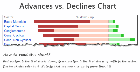
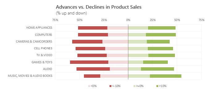
You may have seen this chart in financial newspapers or websites. Shown below, Advances vs. Declines chart tells us how many items have advanced & how many have declined.
When should you use Advances vs. Declines chart?
As you can see, advances vs. declines chart does not give low level details about actual movement of values. Instead, it gives you a sense of what is going on. Use it in below situations:
- To get a feel of how values have changed over time.
- When you are dealing with data that constantly changes (sales, number of customers, defects etc.)
Create Advances vs. Declines chart in Excel
You can easily create this chart in Excel from raw data. Just follow below tutorial.
Step 1: Get the data & arrange it
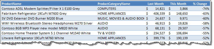
You need at least 4 columns of data – item, category, previous value, current value
Once we have these, calculate % change in 5th column. Arrange data like below:
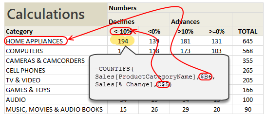
Step 2: Calculate Category-wise summaries
First list all unique categories in a column. Then using COUNTIFS formula, calculate the number of products declining & advancing.
The formula to count number of products going down by more than 10% is,
=COUNTIFS(Sales[category], Category name, Sales[% change], “<10%”)
[Related: Introduction to Excel SUMIFS / COUNTIFS Formulas]
Step 3: Calculate % break-ups for the chart
Once all the numbers are calculated, you can easily calculate the % split.
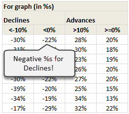
NOTE: Make sure you negate the % values for declines. This will ensure that our chart shows stacked bars on both sides of axis.
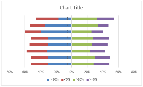
Step 4: Create a stacked bar chart from this data
Once all the numbers are in place, just select them and create a stacked bar chart. Your output should look like below:
Step 5: Adjust chart series order if needed
You may notice that, our stacked chart bars are not in correct order. Excel would have plotted <10% and >10% series before <0% and >0% series. To fix this:
- Right click on the chart
- Go to Select Data
- Now, select the series area
- Using up / down buttons adjust the order of series
- Done!
See this demo to understand:

Step 6: Adjust the colors & format the chart
Unleash your creativity and format the chart as you see fit. Make sure you add legend (otherwise the chart becomes very difficult to read).
And you are done!
Download Advances vs. Declines chart template
Click here to download the chart template. Examine the formulas & chart settings to understand this better.
Do you use Advances vs. Declines chart?
I use variations of this chart often in my dashboards & reports. These charts are very concise and present a lot of information about distribution of changes.
What about you? Do you use advances vs. declines charts? How do you create them? Share your experiences & techniques using comments.
Looking to advance your charting knowledge?
If you want to one up your Excel awesomeness quotient & create kick-ass charts, then you are at the right place. Check out below tutorials & see how deep the rabbit hole goes:
- Visualizing tax changes over time using Excel
- Index Charts – to understand change over time
- Use Box plots to understand distribution of values
- Visualize monthly changes using Pivot Tables + Conditional formatting
Recommended: If all these sound exciting, you will incredibly benefit from our Excel School program, where we teach advanced charting & data analysis skills. Click here to know more & join us.


20 Responses to “Untrimmable Spaces – Excel Formula”
Hi Chandoo,
First of all, HAPPY NEW YEAR!!! Wish you and your family another fruitful year ahead.
To answer your question: Power Query is the best way to trim. 🙂
Btw, if Power Query is not available, then formula would absolutely do... but did you forget to mention also Char 32?
One more question: Is the trailing minus meant to be a negative number? Maybe only the sender knows... 🙂
Cheers,
I just see your PQ way, it is amazing, I think it is the most simple way.
No idea how it did it?
I know these spaces can be a real pain but these days I advise Excel users to learn and use Flash Fill and that will learn what to do pretty quickly.
Highlight range to be cleaned. Then, in Replace, hold down the Alt key and type 0160. Replace with nothing.
I accomplished this by writing a macro to go through all the possible unprintable characters. Looped through the range.
@Steve
Brute force works just as well, its just slower
I use a different method here. First, I will copy the data from Excel and paste it in a notepad. In Notepad, I will do a Find Blanks (Space " ") and Replace (Empty) with nothing.
Then you can copy the data from Notepad and paste it back to Excel which will be a perfect number as you desire.
But Thanks for the formula. Its probably the 2nd out of 8 tricks as Chandoo mentioned. Waiting for the rest among 8 from other users 🙂
Hi....
You don't always need notepad for that. I use the Find/Replace is Excel works just fine.
I don't understand the x's. Why weren't they removed in the formula? Or are they part of some sort of numeric formatting that I'm not familiar with? I saw how you handled the non-breaking spaces and the dashes, but am confused about what role the x's played in all this.
Thanks!
Hi Andrew ,
The xs have been used solely to demarcate the actual data text ; thus , without the x in place at the end of text , as in :
x 4,124,500.00 x
it would be impossible to know that there are unwanted trailing characters , in this case , after the last 0.
These xs are not part of the original data text , nor are they used in the formulae ; they are put in only so that readers can visualize the individual items of data as they are in practice. Think of them as imaginary delimiters.
Oh, that makes sense! Thank you for the explanation. I had a feeling it was something along those lines.
You can type this character using the Keys Alt+0160.
Very useful to replace this Character using Find and Select resource.
For many years, my jobs have included ETL tasks and I built this macro to help long, long ago. I tweak it every now and again. Many co-workers, past and present, have it wired to a button on their toolbar.
Sub Clean_and_Trim()
'CAUTION: Strips leading zeroes -- do not use on zipcodes, etc.
If Application.Calculation = xlCalculationAutomatic Then
Application.Calculation = xlCalculationManual
Revert = 1
ElseIf Application.Calculation = xlCalculationManual Then
Revert = 0
End If
For Each Cell In Selection
For x = Len(Cell.Value) To 1 Step -1
If Asc(Mid(Cell.Value, x, 1)) = 160 Then
Cell.Replace What:=Chr(160), Replacement:=" ", LookAt:=xlPart, MatchCase:=True
End If
If Asc(Mid(Cell.Value, x, 1)) = 32 Then
Cell.Replace What:=Chr(32), Replacement:=" ", LookAt:=xlPart, MatchCase:=True
End If
Next x
If Cell.Value "" Then
Cell.Value = Application.Clean(Application.Trim(Cell.Value))
End If
Next
If Revert = 1 Then
Application.Calculation = xlCalculationAutomatic
ElseIf Revert = 0 Then
Application.Calculation = xlCalculationManual
End If
End Sub
This is awesome! What if you have several characters you need to have removed? What would be the easiest way as I can imagine there are several ways.?
# - 35
$ - 36
- 62
/ - 47
, - 44
. - 46
" - 34
: - 58
This is typical case of a Fitbit data export to Csv file. Each number has CHAR160 as thousand separator.. how smart Fitbit, thank you 😉
By the way, i prefer to copy the character, and use find and replace.
Sometimes it happens if you copy a table from outlook and paste it in excel. When you apply formula on those cells you will get error. What i use to do is
copy one character that looks like space,
select the entire range,
go to Find and replace,
Paste the copied character in Find option
Leave the replace option unfilled..
click on replace all..
All the errors shall be converted in to proper values..
Process looks lengthier.. but it is one of the simplest method
If Clean, Trim, and Substitute, or Find and Replace does not complete the job, I usually enter a value of 1 in an empty cell. Copy the Value of 1, Highlight the range of text numbers, and Paste Special, Values, Multiply. This site is great!
You can use Dose for Excel Add-In that can quickly clean huge data with one click besides more than +100 new functions and features to add to your Excel to save time and effort.
https://www.zbrainsoft.com
Hi,
I have a problem in excel. The sheet attached herewith.
TABLE CONFIG 2/6
A B C D E F G H
1 WEIGHT1 43,599 WEIGH2 62500 WEIGHT3 77000 WEIGHT4 66,500
2 DEDUCTION1 15,000 DEDUCTION1 15,000 TEMP 0 DEDUCTION2 11,005
3 RESULT 58,599 RESULT-1 77,500 RESULT-2 77,000 RESULT-3 77,505
4 RESULT SUBSTRACT 0 0 0
5 REQUIRED VALUE 77,500 77,000 77,505
Note: 1- RESULT (58599) IS TO BE DEDUCTION EITHER FROM D4 OR F4 OR H4 WHICHEVER IS MOST
LEAST CELL AMONG RESULT-1 OR RESULT-2 OR RESULT 3.
2-HENCE, RESULT VALUE $B$3 IS TO BE PRESENTED ON CELL EITHER D4 OR F4 OR H4 WHICHER IS
MOST LEAST VALUE
3-FORMULA =IF(E8<H8,$B$9,IF(E8<J8,$B$9,IF(H8<J8,$B$9,IF(H8<E8,$B$9,IF(J8<H8,$B$9))))))
CREATED ON CELL D4,F4 & H4 DID NOT WORK.
PLS FOR YOUR HELP.
THANK YOU
@R
Why not ask the question in the Chandoo.org Forums
https://chandoo.org/forum/
You can attach a file there