
Comparison is one of the most common things we do with Excel. Naturally, there are so many ways to compare 2 lists of data using Excel. We have discussed various techniques for comparison earlier too,
- Compare 2 lists using conditional formatting
- Even faster way to compare lists
- Compare lists using row differences
Today, I want to share an interesting comparison problem with you.
Lets say you run a small shop which sells some highly specialized products. Now, since your products require quite some training before customers can buy them, you keep track of all product queries and arrange demos.
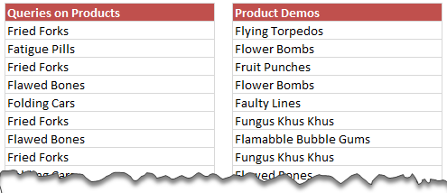
After a hectic week, you are staring at 2 lists. One with product queries, another with product demos.
And you have 2 burning questions,
1. Did we finish all the queries we had?
2. Should I go get some coffee?
Lets answer question number 2. Yes, you can get some coffee. Go, enjoy it now
Back already?!? Good. Now, lets answer the question 1.
Compare 2 Lists Visually using Conditional Formatting
[Note: this article is inspired by Reepal’s comment.]
You would like to highlight the lists as shown below, so that you would know whether each product query is fulfilled or not.
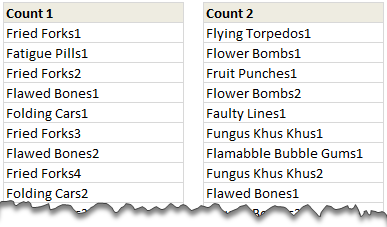
Step 1: Create 2 more lists, with count of products
In order to compare our lists, we need some help. We will create 2 more lists like this:
How do we generate these lists?
Assuming our original data is in B6:B33 and D6:D33,
- In a blank cell (lets say in F6), write =B6&COUNTIF(B$6:B6,B6)
- This gives the count of first product up to that point, ie, Fired Forks1.
- Now drag & fill the formula down until F33
- Do the same in column H, but use the formula =D6&COUNTIF(D$6:D6,D6)
- Fill this until H33
Step 2: Name these new lists
Now that we have created 2 more lists, lets give them names. Select the range F6:F33, go to Formula ribbon and click on “Define Name”. Name the range count1s
Do the same for range H6:H33 and name it count2s
Stpe 3: Apply Conditional Formatting to First List (Product Queries)
Now that we have done all the background work, lets visually compare the data. Select the first list (B6:B33) and go to Conditional Formatting > New Rule
We need to write a rule such that we would highlight all the items in list 1 whenever there is a match in list 2.

The rule is =COUNTIF(count2s,$F6)>0
It means, is the value in F6 present in 2nd list?
in other words, does the first product query has a corresponding product demo?
Set the formatting as you want. Click ok.
Step 4: Apply conditional formatting to Second List
Use the same logic, but this time the rule becomes =COUNTIF(count1s,$H6)
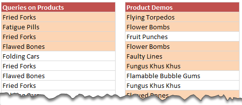
That is all, we have visually compared the two lists.
If you feel like, you can go back for one more cup of coffee.
Download Example Workbook
Click here to download the example workbook – Compare 2 lists visually and play with it. Examine the formulas in columns F & H. Also examine the conditional formatting rules to understand how this works.
How do you compare lists of data?
For me comparison is an everyday task. I rely in several techniques, some quick and dirty, others a bit more elaborate. For quick comparisons, I use either row differences or highlight duplicates rule. For elaborate comparisons, I use COUNTIF, VLOOKUP or other formula based techniques.
What about you? How do you compare lists of values? What techniques and tips you suggest. Please share using comments.
Want to learn Excel Formulas?
If you want to learn Excel formulas so that you can compare, analyze and present better, then please consider joining my Excel Formula Crash Course. This is an 8 hour online training program aimed to make you awesome in Excel formulas. We teach more than 40 every day formulas with loads of real-world examples, practice material & homework.


15 Responses
Hi,
I solved this in a little different way.
We have 2 lists, one starts at A1 and other at B1, both are vertical arrays.
First thing is define 2 named ranges, list1 and list2:
list1 refers to “=OFFSET(Sheet1!$A$1;0;0;SUMPRODUCT(–(Sheet1!$A$1:$A$1000″”));1)”
list2 refers to “=OFFSET(Sheet1!$A$1;0;0;SUMPRODUCT(–(Sheet1!$B$1:$B$1000″”));1)”
this way lists will be dynamically sized when you had or remove elements (you can’t have blanks and you can’t have more than 1000 elements).
Then I use conditional formatting in column A when this formula is true:
“=NOT(ISERROR(MATCH(A1;list2;0)))”
and “=NOT(ISERROR(MATCH(B1;list1;0)))” to list2.
This way we eliminate the need for auxiliary columns or lists.
Hope you like my way! 😀
Nunes
Simple conditional formatting formula.
Assuming lists vertical lists starting in A1 & B1
To highlight just one column (assume B for example)
Conditional formatting>New Rule>by formula
=MATCH(B1,$A$1:$A$99,0)
Set the cell fill to what ever color you prefer & press OK
To highlight both columns repeat with this formula for cell in column A
=MATCH(A1,$B$1:$B$99,0)
This approach doesn’t require named fields or addtl columns
glw
Say I had 1 list in A2:A20 and another in B2:B20.
To format all the items in column A that are repeated in column B I would use the following Conditional Formatting rule.
=IF(ISNA(VLOOKUP(A2,$B$2:$B$20,1,false)),true,false)
All the duplicates are highlighted. It us a very simple example of comparison.
I may be missing something here, but I usually highlight both my lists by holding ctrl eg A1:A20 E10:E40 then choose conditional formatting from the ribbon and then highlight duplicates, and this does it?
Lee, I was perplexed as well. I do the same thing you do with the conditional formating. A drag and click to highlight range and choose highlight duplicates does the trick for me.
I believe these methods are to check if an item from one list also appears in the other list. So if an item mentioned many times in one list if also mentioned in the other list or not.
The Conditional Formatting highlight duplicates feature will do this, but it will also highlight an item if it appears multiple times in the one column or list.
Hi, I would just like to know (if you are willing to share) which image editing program you use to make your image like above, like they are torn apart from bottom? I’ve been looking for long.
@i48998
Chandoo is on Holidays, but Chandoo uses Paint.Net
Paint.net is a free download available at http://www.paint.net/
.
I use CorelDraw/PhotoPaint
.
We both use the Snipping Tool (a freebe with Win Vista/10)
.
We both use Camtasia for doing screen captures to make animated GIFs where you see animation.
Here is how I would accomplish
(1) Define Names: List_1, List_2
(2) =ISNA(MATCH(D4,List_2,0))-1 (Conditional Format formula List_1)
(3) =ISNA(MATCH(D4,List_1,0))-1 (Conditional Format formula List_2)
ISNA will return 1 if NO Match and O if Match by adding a -1 will make: NO Match 0 and Match a -1 which is True
Hi all
this my first Post here
i think we can take Unique List for tow list to know what is not Duplicate By this Array formula
=IFERROR(INDEX($D$6:$D$33,SMALL(IF(ISERROR(MATCH($D$6:$D$33,$B$6:$B$33,0)),ROW($D$6:$D$33)-ROW($D$6)+1),ROWS($J$5:J5))),””)
and this one for Duplicate Value
=IFERROR(INDEX($D$6:$D$33,SMALL(IF(ISNUMBER(MATCH($D$6:$D$33,$B$6:$B$33,0)),ROW($D$6:$D$33)-ROW($D$6)+1),ROWS($J$5:J5))),””)
Don’t forget to Enter This Formula by Pressing Ctrl+Shift+Enter
without wanting to ruthlessly self promote here, I do have an addin that does neatly compare two ranges, not just in columns, so you might want to check that out.
Having said that this is a pretty neat solution if you dont want to be going down the VBA or purchase route. I like it
however, could you not do something with the remove duplicates feature in Excel 2010 and then compare the resulting data set?
Hi, Chandoo! I’ve found yesterday your Excel website… What can I say? It’s just awesome, Excellent. Being a developer for 30 years, more than 15 with Office products, and wow!, how many things I discovered in a couple of hours, and what pretty resolved.
I decided to take the long path of the newbies and read all your examples and write down by myself all of them, and when I arrived to this (the comparison of two lists) I think I’ve found a problem:
a) in “Step 4: Apply conditional formatting to Second List – Use the same logic, but this time the rule becomes =COUNTIF(count1s,$H6)” it should say “Step 4: Apply conditional formatting to Second List – Use the same logic, but this time the rule becomes =COUNTIF(count1s,$H6)>0”, but this is a typing error that I believe all of us here might have discovered and corrected
b) the very problem: I wrote down two different lists, in different ranges, and with different number of elements, I specified the equivalent conditional formats, et non voilá!, I didn’t get what expected. So I downloaded your example book, I checked range names, formulaes, conditional formats and all OK. So I copied -just values- from my book to yours, and I still couldn’t achieve the goal.
I’m using Excel 2010 in spanish, I’m from Buenos Aires (Argentina), and my book is at your disposition whenever you considerate it appropiate.
Thanks in advance for your time, and again my congratulations for your work here.
Best regards.
SirJB7
Comparison of 2 lists visually with highlights
Author: SirJB7 / Date: 11-Dic-2011
Pros: no duplicated tables, no matrix formulaes, no named ranges, no VBA code, just conditional formatting
Cons: not found yet, comments and observations welcome
Features:
a) standard problem: highlights in orange/yellow elements existing in the other list
b) optimized problem: idem a) plus highlights in red/violet first occurrence of elements existing in the other list
Sheet contents:
a) conditional format, 1 rule per list (2 methods used)
A1:A20, first list
B1:B20, second list
a1) range A1:A20, condition =NO(ESERROR(BUSCARV(A1;B$1:B$20;1;FALSO))), format Orange —> in english: =NOT(ISERROR(VLOOKUP(A1,B$1:B$20,1,FALSE)))
a2) range B1:B20, condition =CONTAR.SI(A$1:A$20;B1)>0, format Yellow —> in english: =COUNTIF(A$1:A$20,B1)>0
b) conditional format, 2 rules per list (2 methods used)
D1:D20, first list
E1:E20, second list
b1) range E1:E20, condition 1 =Y(NO(ESERROR(BUSCARV(D1;E$1:E$20;1;FALSO)));COINCIDIR(D1;D$1:D$20;0)=FILA(D1)), format Red —> in english: =AND(NOT(ISERROR(VLOOKUP(D1,E$1:E$20,1,FALSE))),MATCH(D1,D$1:D$20,0)=ROW(D1))
same range, condition 2 and format 2, same as a1)
b2) range E1:E20, condition =Y(CONTAR.SI(D$1:D$20;E1)>0;COINCIDIR(E1;E$1:E$20;0)=FILA(E1)), format Violet —> in english: =AND(COUNTIF(D$1:D$20,E1)>0,MATCH(E1,E$1:E$20,0)=ROW(E1))
same range, condition 2 and format 2, same as a2)
Personally I like the a2) and b2) solutions, I think the formulaes are prettier.
I still don’t know the rules of this website and forum, but it any precept is infringed I’m willing to share the workbook with the solution. If it breaks a rule, I apologize and promise that won’t happen again.
Best regards for all!
Dear All i have a complicated situation…
1. I have two sheets of data Sheet1 and Sheet2 (from various sources) – Both of these contain data matching and Not matching as well..
2. Now for me i need to build an excel where in i need to get sheet 3 with values that are present in a column of Sheet 1.
What ever Sheet 1 doesn’t have i dont want those rows from sheet 2 to be populated into Sheet3.
Can any one help me out.
Hi Team
The above example is to compare partial name from 2 different columns.
If I want to cross check it in a single column. I have both correct and partial correct/match entries in a column. Is there any way I can find both the entries in the column.
Regards