First a Quick Announcement
Our VBA Class enrollments will be closed this Friday (Sep 16). If you want to learn VBA & Excel, please consider joining our course. More than 120 students have already joined us in the second batch and are learning VBA as you read this.
Click here to learn more about the VBA Classes and join us.
Moving on…,
As you may know, Chandoo.org offers quite a few Online Excel training programs. Over the last few weeks, many of you have emailed us and asked which training program is best for your situation. This got me thinking. “It should be easy for YOU to know what is best.”
So today morning, I locked my office room, took out my drawing pad and designed the most comprehensive course recommendation engine. It starts with a survey asking you 12 detailed questions. Then we make you go thru an Excel exam with 15 questions to test your proficiency with the tool. Then the engine would do a lot of calculations and finally recommend a list of training programs that suit you.
Then I threw it out.
Because, it was too complex.
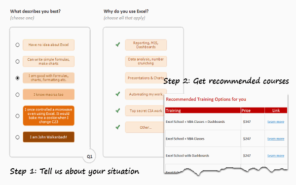
Instead, I made a beautiful Excel workbook that asks you only 2 questions and tells you which training programs are best for you.
How our Training Recommender works?
- You tell us about your Excel skill level
- You tell us why you use Excel
- You get a list of recommended courses
- There is no step 4. I just like 4 bullet points for every thing.

How to get your recommendations?
Simple. Click here to download the tool. Open it using Excel 2007 or above. Just answer the 2 questions to see your recommendations.
How does the Training Recommender Work?
I made a short video explaining how the workbook is constructed. Watch it below or on our Youtube Channel.
Do you like the Training Recommender?
I really enjoyed constructing this. It shows what is possible in Excel.
What about you? Do you like this?
Similar Articles & Ideas
Since I run a small business, I always look for ways to use Excel to enhance areas of my business. Here are some more ideas that you may find helpful.
- Quotation Template made using Excel
- Product Catalog using Excel
- Is Excel School right for me? Assessment Tool
Last but not least…
This is week is the last week to join our ongoing VBA Classes. Next batch will be in 2012.
So go ahead and enroll here.


24 Responses
I’d suggest simply using the subtotal function and filtering the data using the Win/Loss column. You get the same results and the formula is more comprehensible.
@John
That is one option.
There are times however when you want to see the whole data table or a filtered subset and still want to produce summary reports against an unfiltered field.
Is there a particular reason why you are using a comma and the unary (–) operator for the second array in the SUMPRODUCT formula? It seems to work the same if you were to string the arrays together using the asterisk (*). The advantage is that SUMPRODUCT treats the entire string of arrays as a single array.
@Mathew
Your correct, There is no difference.
I thought it may have been easier to explain this method.
Is there a way to do this on a large set of data? As in ~100,000 rows? When I try I get an error because the formula becomes too long. It says the max length of a formula is 8,192 characters. Excel 2010.
How do I incorporate a specific text within a cell for the second array. For instance, – -(C7:C13=”Apple”)
when I chose a specific text the formula does not work.
@RB
I am not sure what is the issue as if I use the sample data in the post the following work fine
Count:
=SUMPRODUCT(SUBTOTAL(3,OFFSET(C7:C13,ROW(C7:C13)-MIN(ROW(C7:C13)),,1)), –(C7:C13=”L”))
Sum:
=SUMPRODUCT(SUBTOTAL(3,OFFSET(C7:C13,ROW(C7:C13)-MIN(ROW(C7:C13)),,1)),(C7:C13=”L”)*(D7:D13))
You may want to check that there are no leading or trailing spaces in your list of Apples
I should have given a better explanation. Heres my situation. I have a column with cells filled with names like Column 1, Column 2, Pier 1, Pier 2, etc. If the cell just contained Pier and searched for that it works. But because it has other characters in the cell its not recognizing the pier. So how can I extract specific characters of a string of text in this formula?
Hopefully this was a better explanation
Hello-
This formula works pretty well for me except that it slow down excel and prevents some of my macros from working. I was wondering if there was a way to program this in VBA so that excel isn’t always trying to recalculate it. I would like to use a push of a button to get it to run then paste in a cell.
Thanks!
I am trying to sum filtered data in a column, but would want to ignore the negative values in the column. How to go about doing this?
@Akshay
Why not just add a filter to that column to only show the values greater than zero?
The negative values are required for reporting purposes, but their effect on the total is distorting the required output. Please advise.
@Akshay
I’d suggest making a post in the Chandoo.org Forums
http://forum.chandoo.org/
Attach a sample file to simplify the task
I have this working for counting and summing, however, I have a list and for the second array, I need a criteria. That is, I’m looking for b13:b200=”01.??.??” or =left((a1,2) or something like that. These types of criteria matches do not appear to work as I get a blank as a result.
Thanks!
@Bob
As your formula b13:b200=”01.??.??” looks like you are trying to check the first day of the month of the range
What about trying Day(B13:B200)=1
Hai Experts,
i understood this formula well and working fine in MS Excel 2013
but when the same am trying to place in google Spreadsheet it shows error as
“SUMPRODUCT has mismatched range sizes. Expected row count: 1. column count: 1. Actual row count: 2014, column count: 1.” and as a result #VALUE! Appears in cell.
Can anyone please help me how would i get it done in Google Spread sheet
or is there any other formula as a substitute for this.
Thank you very much.
thanks for providing this.. but why does excel keeps on prompting Circular referencing in cell D3?
@Vivek
I don’t know
I just downloaded the file and it is working fine and not showing that error
Goto the Formulas, Calculation Options Tab and check that Calculation is set to Automatic
What version of Excel and Windows are you using ?
I know that this forum is for MS Excel, but I am trying to help someone who is working in Google Sheets. The below formula works in Excel but Google Sheets returns:
“SUMPRODUCT has mismatched range sizes. Expected row count: 1. column count: 1. Actual row count: 39000, column count: 1.” and as a result #VALUE! Appears in cell.
This is the same problem asked by Srichirin above. Does anyone know if there is a formula for Google Sheets that will replicate what MS Excel does?
=SUMPRODUCT(SUBTOTAL(3,OFFSET($C$6:$C$39500,ROW($C$6:$C$39500)-MIN(ROW($C$6:$C$39500)),,1)),- -($C$6:$C$39500=H1),($D$6:$D$39500))
Trying to find a SUMPRODUCT formula that counts the word Closed by date for the last 7 days in a filtered list.
=COUNTIF(M:M,”>”&TODAY()-7) works ok for unfiltered count Column M contains Closure dates (blank if open) and Column L is Status Open or Closed
@ Terry
Please ask the question at the Chandoo.org Forums
https://chandoo.org/forum/
Please attach a sample file to ensure a quicker more accurate answer
I used this formula and worked like a charm! But, now I’ve been requested to use it but adding not one but two criteria in the same formula. For instance the sum I was doing added negative and positive numbers. I’ve been asked to use the exact same formula but adding that only positive numbers were considered… any idea on how to do this?
How exactly do you do sum filtered cells when two criteria are need not just one?
Thank you so much brother literally I have been struggling since morning to get the sum of the filtered category, however, after reading your blog attentively i got my solution, so thanks a lot once again.