
Last week we saw a really cool holiday request form made by Theodor.
This week, we will learn how to combine conditional formatting and data validation to create an awesome data entry form.
First see a demo to understand what I mean:

How to create such a data entry form?
Very simple, just grab a cup of coffee (or your favorite fried-nuts-crushed-and-brewed-with-hot-water) and follow my lead.
Step 1: Set up Data Validation
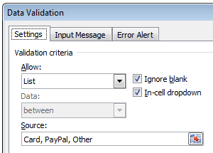
Assuming you need to gather some inputs, like shown above. First thing to do would be setting up data validation rules in a cell so that your users can specify the type of data they are entering. For eg. they can choose card or paypal or other as payment mode and depending on that, enter further details.
To do this, just select the cell and go to Data > Validation. Choose “List” as the rule and give values.
Step 2: Add conditional formatting rules.
Now, based on the selected value, we need to highlight a set of cells.
Assuming all the data to be gathered in cells C4:G4,
Select first two cells (C4:D4), go to Home > Conditional Formatting > New Rule
Here, we need to tell Excel to highlight the C4 and D4 if the type of payment is Card.
So choose the CF rule type as “Use a formula to determine which cells to format” and the check if $B4 is “card”.

Step 3: Add Conditional Formatting rules to other cells (E4:F4, G4)
Using the same logic.
Step 4: Bask in glory!
That is all. There is no step 4. We are done. Finish the coffee or whatever you mixed with hot water. Just save the file and send it to your customer, vendor or boss. Bask in glory as there will be fewer data entry mistakes and more awesome.
Home work: Get Creative and do more
You can use some creativity and make the data entry form even more awesome. For example, you could show a tick mark when the data entry is complete. Also you could highlight only when the cell is blank (ie if the data is already entered, there is no point highlighting)
See what I came up with:

I am not going to tell you how to do the above. That is for you to figure out.
Download Excel Files
Click here to download the excel file with the data entry form example. Play with it to understand how to make similar forms. Become awesome!
And if you can not solve the homework problem, download this file and examine it.
How do you make your data entry forms awesome?
I love data validation. It makes the whole process of gathering valid data dead simple. Also, it is an excellent way to change month or other settings in dashboards. (example 1, 2, 3)
What about you? How do you use Data Validation and other excel features to make your input forms both simple and awesome? Please share your experiences and ideas using comments. Go!
Learn More About Data Validation & Conditional Formatting:
As I said earlier, I really love data validation, conditional formatting features of Excel. They are quite powerful and very useful when working with lots of data. We have very good information about these features on chandoo.org. Start with the below articles to learn more.
- What is Conditional Formatting and how to use it? [Video]
- How to create a simple data validation list?
- 5 tips to become conditional formatting rock star
- More tutorials & tips on conditional formatting, data validation
- Recommended: Join Excel School if you work with data often. You will save a ton of time.


15 Responses
Hey Chandoo,
one more time a great post by you. Although hardcore office enthusiasts often tend to say, as soon as you need a data entry form you should fire up Access I really like your approach in using it in Excel.
Thanks for sharing
Phil
Great and simple post Chandoo. God Bless You!
Hi Chandoo,
Information you provide has always been a great source of inspiration for me to work on excel. Learnt many things from your blog on excel and also implemented in daily job activities.
I have a query relating to data entry forms….
How to make auto addition of rows using formula’s and not using macros. I mean to say, can we create a data entry user form without using macros or data entry form feature / controls and still make a small application which asks the user to input data in sheet (user form), stores in another sheet (database) and provides the summary analysis in the 3rd sheet (dashboard).
I’ve done this on a sort of multi-level basis, tracking a process flow. If the cell in the first column of the row is not blank, it means they’ve started the process, and certain cells need to be filled, and are highlighted if they’re blank. Certain results in some of those cells require filling in others, basically the followup step for that branch in the process. Those in turn have their own required followups. The users are walked across the row of input cells using color, as they work through the multi-week process, and management can tell at a glance (or through filtering the table by color) what is at various stages.
@Raj Kiran: Thank you so much for the love.
There is a feature in Excel called as forms that link to lists or tables. You can use these to gather input data. But these are not as effective as user-forms. Other than that, I am not aware of any non-macro methods to do what you are asking.
@DQK: Very interesting. If possible, please share the file (with dummy data) as it will help our readers appreciate this technique even more.
not possible
Thank you so much for the help
hi, chandoo. thanks for your spread sheets. i am looking for conditional data validation on multiple columns and multiple rows. for eg col 1-country col 2-state col 3-city … row after row.
Thanks for the post.
Could you give me an advise? I can’t find “Edit Formatting Rule” in 2003 Excel Version..
Is it only available with 2007 Version?
Excellent, thanks. Answered my query exactly. Quick and easy to follow – brilliant 🙂
i would like something that is to do with access 2011 please and reply a.s.a.p x
Your post was very helpful. I was banging my head with vbas to accomplish this in excel while there was a simple solution. Thanks 🙂
As usual, your trick was “dead simple” and finished before I could finish my coffee.
I have a query though, instead of highlighting the cells on selection of drop down values, is it possible to block certain cells?
Hello,. I appreciate your spread sheets. I need conditional data validation over several rows and columns. row following row, for example, col 1-country col 2-state col 3-city.