
Sometime in November, I got an interesting E-mail from a gentleman named Guru. The title said “Excel Workshop in Maldives”. In the email, Guru introduced himself and asked me if I can come to Maldives to conduct few Excel workshops for companies and individuals.
I usually neglect such mails as many times the actual training (or big consulting assignment etc.) will not happen. So I replied to him giving my number and asked him to call me. I was surprised to receive his call. After talking awhile, it was clear that Guru is tenacious and would not take No for an answer.
So we set things in motion and thanks to Guru’s perseverance, I ended up boarding a flight to Male on 22nd of January. This is a story of what happened next…,
(note: I traveled with my son & Jo. Business trip for me, beach holiday for them.)
The journey (onward):
Almost all the flights to Male from India leave from either Trivandrum, Chennai or Bangalore. We choose the Trivandrum option because it is a direct flight (other 2 flights have a pit-stop at Colombo, Sri-Lanka). The flight took 75 minutes.
Soon after take-off, all we could see was big-blue Indian Ocean beneath us. About 60 minutes in to the journey and small islands and resorts started appearing. They looked nothing like I have ever imagined. The seas were clear blue or green or a mix. The beaches were pure white. The islands looked lush with greenery. The water villas (houses constructed on water) looked calm and elegant.
The same pattern repeated for next 5-10 minutes in various islands before our pilot announced that we would be touching down at Male international airport.
Male Airport
When I saw Male’s map on Google, I thought the airport could not fit anything bigger than an ATR. But I was surprised when we boarded an Airbus 320 at Trivandrum. But I was in for even bigger surprise when we landed at Male. The airport is as big as many other airports I have seen. In fact, they have an entire island for the airport.
So after getting down and finishing immigration formalities we came out.
A note about visas for Maldives:
Maldives has no prior visa requirements for a majority of countries. Almost anyone can go and get a tourist visa for 30 days. Visit Maldives Visa site for more info.
Guru was waiting for us outside airport. We took a ferry to Male, the capital of Maldives. The airport and capital city are well connected by frequent ferries (one every 10 mins). It takes about 15 mins to reach the city.
Male City – Initial Impressions
I have been to some of the most crowded cities in the world – New York, Mumbai, Hong Kong. But I never saw narrower roads than I did in Male. This is probably the first impression you get too. A majority of Maldivians live in Male. Since the city is a small island, they had to get creative to contain so many people and shops and everything. Some of the impressive ways they manage this:
- Almost all roads are one-ways
- Many buildings are multistory and quite narrow.
- Many elevators are small and can carry 6 people at a time.
- People use bikes or cycles (although you will find a lot of cars, including a BMW that was parked near Sultan Park for the entire duration I was there)
Since I was traveling with family, Guru has arranged accommodation for us in his boss’ house. This was much better than staying in a hotel as my son got more space to play and run.
How my Workshops went?
I had a busy schedule from the moment I landed. On the first day, we conducted a Free Excel Workshop in Aminiya School. This was to get participants to sign-up for our paid workshop.
I choose the topic of Conditional Formatting as it is very close to my heart and the session went very well. We ended up adding few more people to our evening batch.
Later Guru briefed me that I need to conduct 18 hours of Excel training at STELCO (State Electricity Company) and 9 hours at HDC (Hulhumale Development Corp)
We started the training at STELCO next day. We spent the first day discussing Excel overview and writing formulas. The participants were quite friendly and by second day we were cracking jokes and having fun while learning lots of stuff.
Later in the night I conducted a session for individual participants (about 9 of them) again on same topics.
This went for 3 days before we added one more client – FSM (Fuel Supplies Maldives).
What I learned from my workshops?
- Start with Overview: I always assumed that people would know how to use Excel. So my learning plan started with Formulas (that is how it is for Excel School too). But I was surprised to realize that people want to have a good overview of Excel before jumping in to specifics. So after frist day morning, I changed my plan. My first class became “overview of Excel”. In fact, I even added a lesson Zero to Excel School after coming back.
- No plan: Before leaving for Maldives, I made elaborate learning plans for both intermediate and advanced Excel sessions. But after landing there, I realized that it is better to have a loosely structured plan and modify it as per participant’s needs.
- Metaphors are powerful: Often while explaining concepts like namebox, relative vs. absolute references, countif, pivot tables, conditional formatting it was difficult for some participants to understand how they would be relevant. But thankfully, using metaphors I could get my point across
- Talking for 8 hours a day is a lot of work: After talking for more than 8 hours a day for a week, suddenly I respect all my teachers even more.
- Pivot tables excite people: In all my classes, when I demoed pivot tables, I could hear “wow!!! that is so much better” from many participants. They raise the overall curiosity of the class and suddenly everyone is paying attention to know more. (hint: expect more pivot table stuff on chandoo.org too)
Participants’ Response:
We had about 50 people attending the workshops. And a majority of them gave a very high rating (4 or 5 out of 5) for it. Many actually wrote testimonials and praised us for doing it. All 3 companies are hopeful to do a follow-up workshop in a few months.
I also learned a lot of things about Excel while explaining or answering students’ questions.
I had a self-doubt whether I would be able to pull off an in-person training program. Now, I am more confident. I can handle future workshops more easily.
So it was a win-win for all of us.
What we did when I was not teaching Excel?
Despite being a small city, Male has lots of surprises. So we were busy for the first 4 days exploring the city and discovering our way back to home. The best things I liked about Male are,
Walks: You can walk from one end of Male to other end in about 30 mins. So you would start from one ocean front and end up another. Although the streets are narrow, they all have foot-paths. So it is easy to walk, leisurely explore the shops and other attractions, watch other tourists and locals.
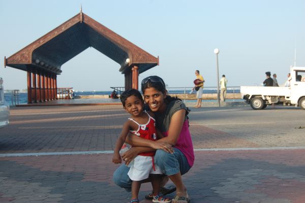
Ocean Front near Jumhoore Maidhan: is a very lively place to sit and watch tourists, enjoy the sun, ocean breeze, play in the park (or watch your kids play).
(Nishanth and Jo in the sun – Near Jumhoore Maidhan, Male)
Food: Lots of restaurants serving authentic Asian, continental and Italian varieties. So many varieties of fish and other sea-food at really affordable prices. We especially liked Thai and sea-food at Lemongrass restaurant near Farhadee Magu (close to Sultan Park).
People: Although we did not interact with many people outside my training hours, what I found is that people are very friendly, helpful and cheerful. Participants of my training program are even more awesome as they showed immense curiosity and sense of humor.
About the beaches:
But many people do not go to Maldives to visit Male. They go because of the spectacular beaches in Maldives.
Unfortunately, due to my busy schedule, we could not get much time to explore various beautiful islands in the archipelago. But we did go to two different islands and they both were mind-blowing.
Hulhumale:
(view from Hulhumale jetty)
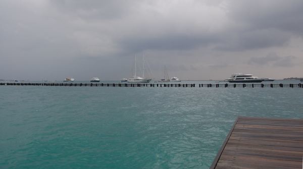
This is an island close to Male. Government of Maldives is developing this island as the mainland Male is very congested. This is where all the new projects are coming up. (and HDC, one of the companies I did training for, is developing the island)
We went to Hulhumale by a ferry on Wednesday (26th of Jan). Hulhumale has lots of beaches (Male has only ocean fronts and one artificial beach). The beaches are very clean, sand is clear white and you can walk almost 200-300 meters in to the water without getting drowned (in some places). We spent the whole evening there.
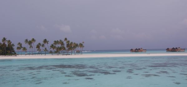
Six Sense Resort – Lankanfushi Island
(view from a water villa – Six Sense Resort – Lankanfushi Island)
A couple of the evening batch students worked at Six Sense Soneva Gili Resort in Lankanfushi Island (one was a training manager and another is a F&B manager). Initially, the training manager tried to arrange a similar workshop at the resort. But they could not make a decision immediately. So we agreed that next time I visit Maldives, I will conduct a workshop at the resort.
But they invited us to spend a day at the resort. Since Maldives is an Islamic country and Friday (and for some companies Saturday) are holidays. So we decided visit the island on Friday (28th). Initially I wanted to say no to the proposal as I was too tired with all the classes. But my wife was keen to enjoy the beaches. So we did go.
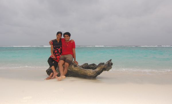
Going there proved to be the best part of the trip. The island and the beaches there are nothing like I have ever seen. The waters, sun, sky and calm resort instantly rejuvenated me. We spent the whole afternoon at the beach. I even swam for a while.
We had some coffee and snacks the restaurant. My son started crying loudly when the restaurant supervisor, a Japanese lady, said hello to him.
(3 of us at the staff canteen – Six Sense resort)
We left the place barely in time to catch the ferry back to Male.
Are you planning to Visit Maldives? A short tourist guide:
When to go?
November to March is a really good time to visit Maldives. It is very sunny and hot through out the year here. So you may want to avoid the summer months (April-June) or Monsoons (July-October).
What to take?
Beach-wear of course. They have showers in Airport too!!! Carry sun-glasses, hats, slippers, cotton clothes.
About Visas:
For a majority of countries, You do not require visa to enter Maldives. You can get a tourist visa for 30 days upon arrival. Visit Maldives Visa information site.
How much it costs to visit Maldives?
Maldivian currency is Rufiya (MVR). You can get 12.75 MVR for each US $.
Almost all the items are imported to Maldives from near-by countries. For this reason, many food items etc are expensive. That said, compared to costs in many developed countries, Maldives is cheap. You can have a really good meal (with sea-food etc.) for about $10.
Some hacks for budget travelers:
- For breakfast, go to Seahouse at the Hulhumale Ferry Terminal. They have breakfast buffet for 65 MVR on all days. You can find all varieties (English, Continental, US, Asian) of breakfast items, juices etc. The best part is, you can watch the ocean, speedboats, soak in sun while enjoying the food for a couple of hours.
- Do not buy milk: It is very expensive here. Instead, you can buy Milk powder and use it for coffee / tea. You can also get yogurt.
- Take a cab: Taxis are un-metered in Male. You can go from anywhere to anywhere by paying just 20MVR. So if you are tired, hail a cab.
- Eat out: There are tons of places through of Male that are cheap and delicious. You can walk in to almost any restaurant and eat food for less than $20.
- No shopping: Since almost everything are imported, you will find the prices to be on higher side for usual shopping items like consumer electronics, clothes, shoes or cosmetics. I was told TVs are cheaper, but carrying one to back home would be a pain.
Closing Thoughts:
We really enjoyed our brief stay at Maldives. I am thankful to Guru and IIPD (the organization Guru works for) for everything they have done to make the training workshops a great success.
Special thanks to STELCO, HDC and FSM for trusting me and giving their time & attention.
I was left with a few hundred Rufiyah by the time we returned to Airport. But I did not give them back to Guru as I know that I would be visiting Male once again. But next time, I hope I could spend a few more hours by the beach too.
Bonus Excel Tip for those of you making this far:
I know you read the travelogue because you want to know more about me. I find it very humbling. So here is a small Excel tip 🙂
Use NETWORKDAYS.INTL() to calculate working days between 2 days with custom weekends:
Often, you may want to find out number of working days between 2 dates. We can use NETWORKDAYS() formula to do this. For eg. NETWORKDAYS(“1-JAN-2011″,”31-JAN-2011”) would tell you the number of working days in Jan (assuming Saturday and Sunday are weekend holidays).
But what if you live in countries like Maldives, where Friday is the weekend. Well, thankfully, you can use the NETWORKDAYS.INTL() formula. This is a new formula introduced in Excel 2010.
So =NETWORKDAYS.INTL(“1-JAN-2011″,”31-JAN-2011”,16) will give you the number of working days in Jan 2011 assuming Friday is a weekend holiday.
But what if you don’t have Excel 2010?
Well, you can use networkingdays() custom UDF instead.


19 Responses
Wow, your description really makes the Maldives sound like a terrific place to visit. Too bad the airfare for me would probably be more than the rest of the trip combined! Who knows though, I may make it there one day yet!
Good post Chandoo — thanks for sharing. I’ve been enjoying your site for the last few years, but this is my first comment/post. I think the workshop lessons learned section of this post is useful for your readers as well. Many of your readers probably provide Excel training to friends/colleagues, either casually or formally, and these bullets are good reminders of what Excel students need to move up the learning curve. Keep the wisdom coming. Cheers, E
Or rather than networkdays or the UDF :-
=SUMPRODUCT(–(MOD(ROW(INDIRECT(E3&”:”&F3)),7)6))
Where E3 is the start Day and F3 is the end day!
(I just replied this exact same thing for Saturdays 2 seconds before this post arrived!)
Totally concur with your feedback on giving Excel classes.
I have to admit that giving such intense workshops in such a beautiful setting does raise the bar for all the rest of us 🙂 God knows I’d love to get back there… albeit for diving 🙂
Hey!! don’t leave your daughter at your in-law’s place next time 🙂
Chandoo,
Great ! This is probably your beginning of a new chapter in your career….Traveling around the world, sharing and empowering people to be awesome in Excel !
Would you say that this is something you love to explore further?
Hi chandoo it’s cool like u
Hi All readers
I came to know about chandoo in MSN (http://education.in.msn.com/news/article.aspx?cp-documentid=4583472) tat was very inspiring; I read that article nearly 3 times. I think I wrote the mail to him after reading his article. I am surprised that he accepted my invitation to come and give training in Maldives.
Then we both designed the training program and I did marketing for that, it was highly challenging for me as it is my first initiative in my office. Off course all the hard work will lead to success but chandoo helped to triple the success. All participants and colleagues are very happy for organizing this workshop.
Few snapshots about chandoo!
1. Affectionate towards family
2. Passionate about excel
3. Cool person
Chandoo all de very best for your future projects
Doesn’t seems you have a bad time in your journey…. 🙂
Congrats!
Greetings from Argentina.
Pablo.
Congrats on the first of many international Excel workshops Chandoo!
Hey Chandoo, if you ever come to New York or New England here in the US, I’d like to hear about it and maybe meet you!
Hi,,
Am a Sri Lankan working in maldives, last couple of months I have been going through your website and it is very impressive your works and creative thing, we thank you for sharing those with us. Unfortunately, for some reason I missed the work shop that you held at Maldives. In fact I called guru by that time it was too late,, I gave my number to guru asking him to call me back,, on your next visit. 🙂
@All… thanks for your comments and love.
@Guru: Thank you so much for your hospitality and care. I am really looking forward to visit the islands once again.
@Ahmed: Sure, we will meet next time I am in Male.
@Matthew: How I would love to do a workshop (or a series) in NY or Seattle. I am trying the find some sponsors and people in US to collaborate. Lets see how it goes.
@Squiggler: Good one! I saw Jeff Weir use the same technique few months earlier.
A lovely part of the world to visit. I went in 2004 for my honeymoon and will never forget the place. Next time I want to stay for much longer!
I wish it was only a 75 minute flight for me. More like 14 hours from the UK but well worth it
I recently read your post on using Choose(Code) vs. nested if statements and I cannot figure out how this function works. Can you please explain. I would have used a vlookup as a secondary step, but would love to know how to combine the formula. Thanks.
It’d be great if someday you came to Peru and visit Machu Picchu. I know you’ll love it. Oh really, Congratulations for your first International Excel.
Greetings to you and your lovely family.
envy … 🙂 I plan to visit maldives this year for honeymoon. Do you have any suggestions? such as the place that must be I visit there?
Dear Cimaja…
ma sister enjyd her honeymoon there…she told me it was nice…she went ther by the help of a good tour operator there…its better u to contact them…and ask them for good resorts…
email id: cooperate@sunnymaldives.com
or visit there site
website: http://www.sunnymaldives.com/