
This is a guest post by Daniel Ferry of Excelhero.com.
 Have you ever wanted to fetch live stock quotes from excel? In this post we will learn about how to get stock quotes for specified symbols using macros.
One method that has worked well for my clients can be implemented with just a few lines of VBA code. I call it the ActiveRange.
An ActiveRange is an area on a worksheet that you define by simply entering the range address in a configuration sheet. Once enabled, that range becomes live in the sense that if you add or change a stock symbol in the first column of the range, the range will automatically (and almost instantly) update. You can specify any of 84 information attributes to include as columns in the ActiveRange. This includes things such as Last Trade Price, EBITDA, Ask, Bid, P/E Ratio, etc. Whenever you add or change one of these attributes in the first row of the ActiveRange, the range will automatically update as well.
Sound interesting, useful?
In this post, you can learn how to use excel macros to fetch live stock quotes from Yahoo! Finance website. It is also going to be a crash course in VBA for the express purpose of learning how the ActiveRange method works so that you can use it yourself.
Download Excel Stock Quotes Macro:
Click here to download the excel stock quotes macro workbook. It will be much easier to follow this tutorial if you refer to the workbook.
Background – Understanding The Stock Quotes Problem:
The stock information for the ActiveRange will come from Yahoo Finance. A number of years ago, Yahoo created a useful interface to their stock data that allows anyone at anytime to enter a URL into a web browser and receive a CSV file containing current data on the stocks specified in the URL. That’s neat and simple.
But it gets a little more complicated when you get down to specifying which attributes you want to retrieve [information here]. Remember there are 84 discreet attributes available. Under the Yahoo system, each attribute has a short string Tag Code. All we need to do is to concatenate the string codes for each attribute we want and add the resulting string to the URL. We then need to figure out what to do with the CSV file that comes back.
Our VBA will take care of that and manage the ActiveRange. Excel includes the QueryTable as one of its core objects, and it is fully addressable from VBA. We will utilize it to retrieve the data we want and to write those data to the ActiveRange.
Before we start the coding we need to include two support sheets for the ActiveRange. The first is called “YF_Attribs”, and as the name implies is a list of the 84 attributes available on Yahoo Finance along with their Yahoo Finance Tag Codes. The second sheet is called, “arConfig_xxxx” where xxxx is the name of our sheet where the ActiveRange will reside. It contains some configurable information about the ActiveRange which our VBA will use.
All of the VBA code for this project will reside inside of the worksheet module for the sheet where we want our ActiveRange to be. For this tutorial, I called the sheet, “DEMO”.
Writing the Macros to Fetch Stock Quotes:

Press ALT-F11 on your keyboard, which will open the VBE. Double click on the DEMO sheet in the left pane. We will enter out code on the right. To begin with, enter these lines:
Private rnAR_Dest As Range
Private rnAR_Table As Range
Private stAR_ConfigSheetName As String
Always start a module with Option Explicit. It forces you to define your variable types, and will save you untold grief at debugging time. In VBA each variable can be one of a number of variable types, such as a Long or a String or a Double or a Range, etc. For right now, don’t worry too much about this – just follow along.
Sidebar on Variable Naming Conventions
Variable names must begin with a letter. Everyone and their brother seems to have a different method for naming variables. I like to prefix mine with context. The first couple of letters are in lower case and represent the type of the variable. This allows me to look at the variable anywhere it’s used and immediately know its type. In this project I’ve also prefaced the variables with “AR_” so that I know the variable is related to the ActiveRange implementation. In larger projects this would be useful. After the underscore, I include a description of what the variable is used for. That’s my method.
In the above code we have defined three variables and their types. Since these are defined at the top of a worksheet module, they will be available to each procedure that we define in this module. This is known as scope. In VBA, variables can have scope restricted to a procedure, to a module (as we have done above), or they can be global in scope and hence available to the entire program, regardless of module. Again we are putting all of the code for this project in the code module of the DEMO worksheet. Every worksheet has a code module. Code modules can also be added to a workbook that are not associated with any worksheet. UserForms can be added and they have code modules as well. Finally, a special type of code module, called a class module, can also be added. Any global variables would be available to procedures in all of these. However, it is good practice to always limit the scope of your variables to the level where you need them.
In that vein, notice that the three variables above are defined with the word Private. This specifically restricts their scope to this module.
Every worksheet module has the built-in capability of firing off a bit of code in response to a change in any of the sheet’s cell values. This is called the Worksheet_Change event. If we select Worksheet from the combo box at the top and Change in the other combo box, the VBE will kindly define for us a new procedure in this module. It will look like this:
![]()
End Sub
Notice that by default this procedure is defined as Private. This is good and as a result the procedure will not show up as a macro. Notice the word Target near the end of the first line. This represents the range that has been changed. Place code between these two lines so that the entire procedure now looks like this:
The Heart of our Excel Stock Quotes Code – Worksheet_Change()
ActivateRange
If Worksheets(stAR_ConfigSheetName).[ar_enabled] Then
If Intersect(Target, rnAR_Dest) Is Nothing Then Exit Sub
If Target.Column <> rnAR_Dest.Column And Target.Row <> rnAR_Dest.Row Then
PostProcessActiveRange
Exit Sub
End If
ActiveRangeResponse
End If
End Sub
That may look like a handful but it’s really rather simple. Let’s step through it. The first line is ActivateRange. This is the name of another sub-procedure that will be defined in a moment. This line just directs the program to run that sub, which provides values to the three variables we defined at the top. Again, since those variables were defined at the top of the module, their values will be available to all procedures in the module. The ActivateRange procedure gives them values.
Next we see this odd looking fellow:
If Intersect(Target, rnAR_Dest) Is Nothing Then Exit Sub
All this does is check to see if the Target (the cell that was changed on the worksheet) is part of our ActiveRange. If it is the procedure continues. If it’s not, the procedure is exited.
The next line checks to see if the cell that was changed is in the first column or first row of the ActiveRange. If it is, the post processing is skipped. If the change is any other part of the ActiveRange, another sub-procedure (defined below) is run to do some post processing of the retrieved data, and then exits this procedure.
If the cell that changed was in the first column or the first row, the program runs another sub-procedure, called ActiveRangeResponse, which is also defined below. ActiveRangeResponse builds the URL for YF, deletes any previous QueryTables related to the ActiveRange, and creates a new QueryTable as specified in our configuration sheet.
That’s it. The heart of the whole program resides here in the Worksheet_Change event procedure. It relies on a number of other subprocedures, but this is the whole program. When a change is made in the ActiveRange’s first column (stock symbols) or its first row (stock attributes), ActiveRangeResponse runs and our ActiveRange is updated.
Understanding other sub-procedures that help us get the stock quotes:
So let’s look at those supporting subprocedures. The first is ActivateRange:
stAR_ConfigSheetName = “arConfig_” & Me.Name
Set rnAR_Dest = Me.Range(Worksheets(stAR_ConfigSheetName).[ar_range].Value)
Set rnAR_Table = rnAR_Dest.Resize(1, 1).Offset(1, 1)
Worksheets(stAR_ConfigSheetName).[ar_YFAttributes] = GetCurrentYahooFinancialAttributeTags
End Sub
Again, all this does is give values to our three module level variables. In addition it builds the concatenated string of YF Tag Codes required for the URL. It does this by calling a function that I’ve defined at the very bottom of the module, called GetCurrentYahooFinancialAttributeTags.
The next subprocedure is ActiveRangeResponse:
Dim vArr As Variant
Dim stCnx As String
Const YAHOO_FINANCE_URL = “http://finance.yahoo.com/d/quotes.csv?s=[SYMBOLS]&f=[ATTRIBUTES]”
vArr = Application.Transpose(rnAR_Dest.Resize(rnAR_Dest.Rows.Count – 1, 1).Offset(1))
stCnx = Replace(YAHOO_FINANCE_URL, “[SYMBOLS]”, Replace(WorksheetFunction.Trim(Join(vArr)), ” “, “+”))
stCnx = Replace(stCnx, “[ATTRIBUTES]”, Worksheets(stAR_ConfigSheetName).[ar_YFAttributes])
AddQueryTable rnAR_Table.Resize(UBound(vArr)), “URL;” & stCnx
End Sub
Notice that here we have variables defined at the top of this procedure and consequently their scope is limited to this procedure only. This means that we could have the same variable names defined in other procedures but those variables would not be related to these and would have completely different values.
Next notice that we have defined a constant. This is good practice, as it forces us to specify what the constant value is by naming the constant. I could have just used the value where I later use the constant, but then the question arises as to what is this value and where did it come from. Here I have named the value, YAHOO_FINANCE_URL, removing all doubt as to its purpose.
The next line is this:
vArr = Application.Transpose(rnAR_Dest.Resize(rnAR_Dest.Rows.Count - 1, 1).Offset(1))
and it deserves some explanation. Let me back up by saying that whenever we write or read multiple cells from a worksheet we should always try to do it in one go, rather than one cell at a time. The more cells involved the more important this is. Otherwise we pay a massive penalty in processing time. One of the best optimization techniques available is to replace code that loops through cell reads/writes and replace it with code that reads/writes all the cells at once. It can literally be hundreds to thousands of times faster.
Here we are interested in getting the list of all of the stock symbols in the first column of the ActiveRange. So how do we get them in one shot? We use something called a variant array. Notice that we defined vArr at the top of this procedure. A variant array is a special kind of variable that holds a list of values and it DOES NOT CARE what variable types those values are. This is important when retrieving data from a sheet because the data could be numbers, text, Boolean (True or False), etc. Variants are powerful, but they are much slower than other variable types, such as a Long for numeric data for example. However, in the case of retrieving or writing large chunks of data from/to a sheet the slight penalty of the variant is dwarfed by the massive increase in the speed of data transfer.
It’s very simple to retrieve range data (regardless of the size) into a variant array. All you do is:
v = range
where v is defined as a variant and range is any VBA reference to a worksheet range. And magically all of the values in that range are now in v. Note that v is not connected to the range. A change in any of v’s values does not propogate back to the range, and likewise a change to the range does not make it’s way to v all by itself. v will ALWAYS be a two-demensional array. The first dimension is the index of the rows, the second dimension is the index of the columns. So v(1,1) will refer to the value that came from the top left cell in the range. v(6,9) will hold the value that came from the cell in the range at row 6 and column 9.
For most circumstances this two-dimensional format is fine. But we are only retrieving one column of stock symbols. The procedure will still give us a two-dimensional array, with the column dimension being only 1 element wide. This is a shame because VBA has a wonderful function called Join that allows you in one step (no loop) to concatenate every element of an array into a string. You can even specify a custom string to delimit (go in-between) each element in the output string. The problem is that Join only works on single dimensioned arrays 🙁
But there’s always a way, right? We can use the Application.Transpose method on the 2-D array and presto we get a 1-D array. The rest of the line just specifies what range (the stock symbols) to grab.
The next two lines are:
stCnx = Replace(YAHOO_FINANCE_URL, "[SYMBOLS]", Replace(WorksheetFunction.Trim(Join(vArr)), " ", "+"))
stCnx = Replace(stCnx, "[ATTRIBUTES]", Worksheets(stAR_ConfigSheetName).[ar_YFAttributes])
Again a handful, but all we are doing here is replacing the monikers, [SYMBOLS] and [ATTRIBUTES] in the YAHOO_FINANCE_URL constant with the list of stock symbols (delimited by a plus sign) and the string of attributes.
In the final line of the procedure:
AddQueryTable rnAR_Table.Resize(UBound(vArr)), "URL;" & stCnx
we are running another subprocedure called, AddQueryTable and we are telling it where to place the new QueryTable and providing the connection string for the QueryTable, which in this case is the YF URL that we just built.
Nothing unusual happens in the AddQueryTable sub. It just deletes any existing AR related QueryTables and adds the new one according to the options in the configuration sheet.
The PostProcessActiveRange sub is interesting:
If rnAR_Dest.Columns.Count > 2 Then
Application.DisplayAlerts = False
rnAR_Table.Resize(rnAR_Dest.Rows.Count).TextToColumns Destination:=rnAR_Table, DataType:=xlDelimited, Comma:=True
Application.DisplayAlerts = True
Worksheets(stAR_ConfigSheetName).[ar_LocalTimeLastUpdate] = Now
End If
End Sub
Processing Yahoo Finance Output using Query Table & Text-Import Utility:
As mentioned before the data from YF comes back as a CSV file. The QueryTable dumps this into one column. If you were only retrieving one attribute for each stock this would be fine as is. However, two or more attributes is going to result in unwanted commas and multiple attribute values squished into the first column of the QueryTable output. Unfortunately this is poor design by Microsoft, especially when you consider that the QueryTable does not behave like this when it is retrieving SQL data or opening a Text file from disk. You can actually specify this operation to be a text file and it will properly spread the output over all of the columns. To do so, you specify the disk location as being the URL of the YF CSV file, but as Murphy would have it, it’s unbelievably slow and pops up a status dialog as it slowly retrieving the CSV. Using the URL instruction instead of the TEXT instruction at the beginning of the connection string is incredibly fast in comparison, but dumps all of the data into the first column.
So what to do? We’ll just employ Excel’s built-in TextToColumns capability and bam, our data is where we want it.
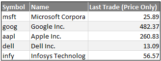
Our finalized stock quotes fetcher worksheet should look like this:

Download Excel Stock Quotes Macro:
Click here to download the excel stock quotes macro workbook. It will be much easier to follow this tutorial if you refer to the workbook.
Final Thoughts on Excel Stock Quotes
The ActiveRange technique is quite versatile. It can be implemented with other data sources such as SQL, or even lookups to other Excel files, or websites.
In this example it provides a nice way to easily track whatever stocks you may have interest in and up to 84 different attributes of those stocks. You can enable and disable the activeness of the ActiveRange on the fly. You can set the AR to AutoRefresh the data at periods that you set or to not refresh at all.
This is a basic implementation. For example, changing the AutoRefresh setting will have no effect until a new QueryTable is built. That won’t happen until you also add or change a stock symbol or add or change an attribute. An easy enhancement would be to add a little code to the arConfig_DEMO code module to respond to changes to the ar_AutoRefresh named range cell.
Another enhancement would be to eliminate the slight flicker of the update by moving the QueryTable destination to the arConfig_DEMO and then doing the TextToColumns with the destination set to the DEMO sheet. In an effort to simplify this tutorial I have left these easy enhancements as an exercise for you to implement.
Have a question or doubt? Please Ask
Do you have any questions or doubts on the above technique? Have you used ActiveRange or similar implementations earlier? What is your experience? Please share your thoughts / questions using comments.
I read Chandoo.org regularly and will be monitoring the post for questions. But you can also reach me at my blog:
Further References & Help on Excel Stock Quotes [Added by Chandoo]
- Fetching Stock Quotes using Research Pane
- Stock Portfolio Tracker using Google Docs
- QueryTable Object Model & Properties
- Using QueryTable to Generate Dynamic Reports
- Yahoo Finance API Documentation & Example
Excel Hero is dedicated to expanding your notion of what is possible in MS Excel and to inspiring you to become an Excel Hero at your workplace. It has many articles and sample workbooks on advanced Excel development and advanced Excel charting.


207 Responses
how do I add attributes? when I add c8, with auto-refresh checked, it restores to ONLY the original attributes … I tried WS protection and this caused VBA errors. Thanks. Doug.
Did you ever get an answer or fix to this?
doug churchill says:
June 2, 2010 at 10:31 am
how do I add attributes? when I add c8, with auto-refresh checked, it restores to ONLY the original attributes … I tried WS protection and this caused VBA errors. Thanks. Doug.
Sorry, never mind, I figured it out after reading all the posts. Thankfully it works!
Well, Daniel, those who learned a lot of programming with this post salute you !
Must say, I do process ranges out of a SQL query, and from plain vanilla sheets as well, and every time I use a cycle (while, for) to calculate other related cells once I retrieved the query result, with a ActiveCell.Offset at the end, to go to the next line.
It worked nice, but it does take a long to retrieve and calculate the info.
You saying this can be done faster, well, definitively is something I must look into….
Any other tip for this behavior? should I leave this to those who actually know what they’re doing? 🙂
Rgds.
Martin
The workbook is nice, but I can only get stock quotes for the companies you’ve chosen.
If I want to return data for another company, how can I figure out its stock symbol?
Nice workbook. Doesn’t look like it is any easier than just setting up web queries though.
@doug churchill –
Are you adding the c8 attribute via entering “After Hours Change (Real-time)” in the first row of the ActiveRange? In the sample for this article that would be row 6 of the DEMO sheet. I just tried this with AutoRefresh checked and it worked perfectly. The fact that you mentioned this attribute by Tag Code makes me think that you tried to add it some other way. Let me kow – I want it to work for you.
@Martin –
Nah, do it yourself! From what you describe it sounds like your loop is interacting with the worksheet too much, and this is the reason for the slow performance on you SQL result set processing. Remember, as discussed in this article, try to limit the number of times you write or read to the worksheet cells. Writing to 1,000 cells in one go takes about as much time as writing to one cell. The variant array is your friend.
@JP –
Doing stock symbol lookups for a given company was outside the scope of this teaching workbook. Agreed that would be a nice feature to add as an enhancement. In the meantime, you can lookup the symbols for virtually any stock at:
http://finance.yahoo.com/lookup
Just start typing the name of a company in the Get Quotes box near the top of the page and it will quickly zero in on that company AND give you its stock symbol. Then just enter that stock symbol into the first column of the ActiveRange on my sample workbook.
Regards to all,
Daniel Ferry
excelhero.com
@Steve-O:
The initial setup is more involved. But after that I think it’s way easier. I’d like to see a webquery where you can on the fly change precisely which companies you want to track and which attributes. This method allows you to do that instantly, with precision.
Besides that though, the point of the exercise is to learn something about VBA programming. The techniques acquired can be used in an infinite number of ways when programming.
Regards,
Daniel Ferry
excelhero.com
Daniel:
I appended it (c8) to arConfig_DEMO:b7 …. it resets to original tags …
Then, as per your comment, I pasted … After Hours Change (Real-time) … to cell g6 as you suggested with auto-refresh checked … no help.
I cannot find where it gets the fields from that you set in arConfig_DEMO:b7
Tks. Doug
@doug churchill –
Ah… B7 is just there for the sake of demonstration. It actually should not be as it is not intended for alteration by the user. Don’t change this as it will have no effect, as you found.
BUT, if you look at B4 on the configuration sheet you will notice that the ActiveRange is defined to end at column F. Go ahead and change this to include whatever columns you plan on displaying on the DEMO sheet. Or, you can just pick the attribute from the dropdowns that already exist in columns B through E of the Demo sheet.
Regards,
Daniel Ferry
excelhero.com
Daniel:
Here is some help for you as mentinoed in the Steve-O response
‘I’d like to see a webquery where you can on the fly change precisely which companies you want to track and which attributes. This method allows you to do that instantly, with precision.’
try this …. cell a2 in the SS … as well as copy/paste symbols in a7 on down.
http://www.gummy-stuff.org/Yahoo-data.htm
Daniel:
Here is some help for you as mentioned in the Steve-O response
‘I’d like to see a webquery where you can on the fly change precisely which companies you want to track and which attributes. ‘
try this …. cell a2 in the SS … as well as copy/paste symbols in a7 on down.
http://www.gummy-stuff.org/Yahoo-data.htm
Daniel : when placing bby (BEST BUY) in column A, we get name ‘Best Buy Co.’ in column b and ‘inc’ is now in column c … thereby pushing all other data fields one extra column to the right, incorrectly ….
I got your drop-downs to work …. I have a couple more good EXCEL links you might like regarding this type of process i will go find for you.
Thanks again.
‘
@doug churchill –
You have discovered a bug at Yahoo!
It turns out that when you specify the Name attribute to be the first column returned, Yahoo Finance makes a mistake and fails to enclose within quotation marks the text that represents the name of the company. Interestingly, if any numeric attribute comes before the Name attribute, YF gets it right and DOES enclose the name within quotation marks.
So why does this matter? Some securities have a comma in their name (Best Buy, Inc.) and when Excel’s TextToColums function is invoked it correctly parses the Comma Separated File on the commas – which causes a problem in this case. When the text is enclosed in parentheses, this is not a problem.
So there are two fixes for this:
1.) Don’t use the Name attribute in the first column.
2.) Download the new version of the program that I have updated to handle this eventuality. Chandoo has kindly updated the normal link so that it now points to the new file. If you are interested, the fix for this is entirely in the PostProcessActiveRange() sub, and is well documented.
.
.
.
On another note, thank you for the link to the gummy-stuff workbook. However, that implementation is not coded very well. The VBA is an absolute mess. And worse, it continually adds new QueryTables to the workbook. If you look at the Data Connections, you will notice that it already has over a hundred! And this continues to grow as it’s used. I would not recommend that workbook as a source to learn from. QueryTables are powerful and useful, but readers should take the time to learn how to use them correctly.
Regards,
Daniel Ferry
excelhero.com
Why not use google finance. Just load their api into the app and away you go.
This same methodology you can use excel to search for jobs by scraping data from indeed.com
Hi Daniel,
Thanks for the tutorial.
Very clever way to deal with the comma in the company name.
However, Yahoo also messes up with some numeric attributes (Last Trade Size) for values greater than 1,000. I’ve lookup Berkshire Hathaway A (BKR-A) to confirm that prices aren’t affected.
Sébastien
@Sebastien Labonne –
Your comment peaked my interest. Berkshire Hathaway A works for me. I noticed in your comment that you listed the stock symbol as bkr-a, but the symbol is actually brk-a. I looked it up on the YF website.
.
Using brk-a, it is returning $104,950.00, which is the correct price at the moment. Is it possible that you had the symbol letters reversed when you tried it?
.
It seems to work fine, even with such a gargantuan stock. 🙂
.
Regards,
Daniel Ferry
excelhero.com
Daniel,
.
There was indeed a typo in my comment with the ticker.
.
The “Last Trade Size ” attribute still looks problematic however. I stopped the code at the PostProcessActiveRange procedure and I see some extra commas.
.
Sebastien
.
Chandoo, the email notification for new comments doesn’t seem to work.
Great tutorial, I only have one question: has anybody had any luck getting the after hours (real-time) attribute to work. I was able to choose it from the drop down menu on the Demo, I was also able to add it to the gummystuff work book but to no avail. Both work books returned an NA-NA value no matter what stock symbol I entered.
Thanks in advance:
Juan
Thanks for the tutorial, I only have one question. In the DEMO sheet that you gave us you say:
Be sure to include a configuration worksheet called, “arConfig_xxxx” where
‘ xxxx is the name of this worksheet. The config sheet must contain the following
‘ named ranges:
‘ ar_enabled (can be True or False)
‘ ar_range (the range on this sheet of the ActiveRange, i.e. a6:f50
‘ ar_AutoRefresh (can be True or False)
‘ ar_interval (an integer representing minutes between refreshes)
‘ ar_YFAttributes (a string of tags for Yaho Finance Attributes)
My question is where do I put that in the arConfig_DEMO? do I just type “ar_enabledtrue” or something like that? Do I need to put a space? Do I need to tab then enter?
Also when I changed the value so I have more area to place attributes the drop down menu does not show, any thoughts on what I am doing wrong?
Dear Friend
i want to change refresh time from 1 min to 1 sec in your activerange_yahoofinance excel sheet. Please give me guideline or update sheet with 1 sec refresh interval.
Thanks in advance.
Great demo, thanks a million!
For those who have problems converting decimals from beeing seperated by “.” (Point) to “,” (Comma)
Modify the TextToColumns call like this:
rnAR_Table.Resize(rnAR_Dest.Rows.Count).TextToColumns Destination:=rnAR_Table, DataType:=xlDelimited, Comma:=True, DecimalSeparator:=”.”
The workbook is very nice and useful, but how can I get stock quotes for the companies having numarical symbol like 14050615.002067 ?
Thanks
scj
The workbook is very nice and use ful, but how can I get stock quotes for the companies having numerical symbols like 14050615.002067.
Thanks in advance:
scjain
Does this macro workbook get around Yahoo’s limit on how many (about 200) different symbols you can retrieve data on at once.
I am attempting to build a workbook that will require retrieving quotes for over 200 securities. Others have gotten around this through clever macros, e.g. http://www.greenturtle.us/index.htm and especially http://www.gummy-stuff.org/Yahoo-data.htm, but I have experienced other problems with their macros and would prefer to go through the process of building my own.
If there is any way you could update this macro to deal with the quote limit issue (if it already doesn’t, I’ll test it later today), as I’m sure it’s fairly straightforward for someone with a background in VBA, it would be extremely helpful to me and I’m sure many others as well.
Thanks in advance.
Just tested your macro workbook and was only able to extend the ActiveRange through row 174.
–
Symbols entered below row 174 are not functional. I presume this is due to Yahoo’s quote restriction and not the macro itself (e.g. maybe I need to change some parameter?). I’ll look more at it, but am really hopeful that you’ll be able to come up with a fix for this limitation.
–
If you need some profit incentive, I’m not opposed to compensating you (or anyone else who’s ambitious enough to tackle the problem) for your work. Let me know.
–
Thanks.
how to view stock quotes for numarical symbols
scj
In name column, some of the company names are truncated such as Verizon (VZ), Microsoft (MSFT), Exon Mobil Corporation (XOM), and others. All the names end up being 16-17 characters. On the Yahoo web page they are complete. Can they be lengthened to be more complete?
Thanks
@Sebastien Labone, @Juan Ramirez, @scjain, @subhash jain, William –
Unfortunately the Yahoo Finance interface used in this application has several shortcomings and bugs. You have found some and there are likely others. These things cannot really be fixed on the Excel side of data request. It would be nice if Yahoo got around to fixing these problems. For the vast majority of uses, the YF returns what is expected, but there is room for improvement.
@Michael – Good tip on the decimal-comma replacement!
@Chandresh Chaturvedi – I’m sorry but the QueryTable built into Excel and leveraged by this application only allows for updates on a schedule of minutes, not seconds. The quickest interval is one minute. The longest interval allowed is 32767 minutes. Setting it to zero turns off the update. It is too bad tha MS chose to impliment it this way, which does not allow finer control of the QueryTable update interval.
@Emerson – Please have a look at my application development services and then contact me if you would like to:
http://www.excelhero.com/blog/2010/06/excel-business-application-development-services.html
Regards to all,
Daniel Ferry
excelhero.com
I am getting an odd problem (running Excel 2000, which might explain it). Downloaded the latest file from this page. Loaded it and the first row (row 7) does not copy across. The auto refresh works, in column B, but the data will not copy across (columns C thru F) unless I change a symbol in column A. Similarly, the time does not update. Is there a function or method missing from Excel 2000? Each time I change the ticker, the older data is copied across to columns C thru F, then the new data refills column B from the web.
Any ideas on fixing?
John
Really impressive work in Excel. Way beyond my understanding, but I’m trying. I want to retrieve the Dividend Yield instead of the 52 Week Low Amount. So I tried changing the string nl1rjn to nl1ryn (on the ar_ConfigDEMO sheet). It doesn’t work, keeps changing it back to ml1rjn and retrieving the same fields. Is there something else I have to change? Thanks in advance for any help.
When I went to implement the indexes to use within my financial file as the MSN Stock Quotes quit working within the file, it didn’t want to handle 1 or 2 of them properly and pushed the data out additional columns via the TextToColumn feature. As such, I ended up using Do While statement, Split and Instr functions, use the count argument within the Replace function, and use the If, Then Else statement all within the block of:
For i = LBound(vArr) To UBound(vArr)
Do While UBound(Split(vArr(i, 1), “,”)) + 1 > rnAR_Dest.Columns.Count – 1
If InStr(1, vArr(i, 1), “, “) = 0 Then
vArr(i, 1) = Replace(vArr(i, 1), “,”, ” “, , 1)
Else
vArr(i, 1) = Replace(vArr(i, 1), “, “, ” “, , 1)
End If
Loop
Next i
Again, this isn’t a perfect resolution and it may not work in all cases such as if there are commas within either the numbers for those languages that use the comma in place of the period for the decimal portion of the number OR for those items that has a comma within the string of a particular field.
As for the original macro that’s in the “Change” event of the worksheet, I moved all of those commands into another newly created private procedure called “UpdateData”, so as to be able to call onto that procedure from multiple locations. As for me, I not only plan on having such data updated when there is data modified on that worksheet, but will have it updated by another means, which I haven’t fully decided as I want it to be as efficient as possible (least amount of work to have to do), but yet, I also don’t want to have it take up too much processing time either for too often of a time period.
See below.
Private Sub Worksheet_Change(ByVal Target As Range)
UpdateData
End Sub
Private Sub UpdateData()
ActivateRange
If Worksheets(stAR_ConfigSheetName).[ar_enabled] Then
If Intersect(Target, rnAR_Dest) Is Nothing Then Exit Sub
If Target.Column rnAR_Dest.Column And Target.Row rnAR_Dest.Row Then
PostProcessActiveRange
Exit Sub
End If
ActiveRangeResponse
End If
End Sub
Emerson,
For your issue of needed to update more stock data, maybe you can create another range variable that is for a current range, which then have it broken down into groups of 150 rows at a time until you have done all of the rows you needed. Not completely sure if this will work, but it’s definitely worth a shot.
Just to the above, I just realized I needed to make a modification for the Target range variable, which I made the following adjustments.
Private rngTarget As Range
‘
Private Sub Worksheet_Change(ByVal Target As Range)
Set rngTarget = Target
UpdateData
End Sub
Private Sub UpdateData()
ActivateRange
If Worksheets(stAR_ConfigSheetName).[ar_enabled] Then
If Intersect(rngTarget, rnAR_Dest) Is Nothing Then Exit Sub
If rngTarget.Column rnAR_Dest.Column And rngTarget.Row rnAR_Dest.Row Then
PostProcessActiveRange
Exit Sub
End If
ActiveRangeResponse
End If
End Sub
Ken,
To make the adjustment, go to your data worksheet, which if you need to have additional columns, you can copy the header cell of one column to the other columns. You then adjust your range on the configuration worksheet. Once you do that, you then make your selection from the drop down list that’s in each of the header row of the different columns. The letters will then automatically adjust on the configuration page. This all assumes of course you have macros enabled and the EnableEvents property of the application is not set to False.
One thing to help speed up the process is to set the workbook’s calculation mode to “xlManual” during the duration of the macro but then have it set back to the user’s setting at the end of the macro.
I have used this method many of times to speed up the process including one case that took an hour to update via a query program with Excel in xlAutomatic calculation mode, but when it was done while in xlManual mode, it took less than one minute to process that same query and data.
Here’s the sad thing about that one case, it had very little calculations involved in it. You would normally that would only be true if there were a lot of calculations within a single workbook, but that just wasn’t the case as I have had workbooks with 100’s times more calculation intensive than that one workbook did have. What it was, that single workbook was getting calculated for every time a single cell was getting modified, thus the workbook was getting re-calculated at least 1,000’s of times within a single query update.
To get stock ticker symbols, you can get it from Yahoo Finance Lookup site at http://finance.yahoo.com/lookup
As for changing to 1 second, I wouldn’t recommend that anyhow as that can cause tremendous other issues. I know things are getting to be faster and faster, but still not that fast yet.
Daniel:
doug churchill posted, June 2: “when placing bby (BEST BUY) in column A, we get name ‘Best Buy Co.’ in column b and ‘inc’ is now in column c … thereby pushing all other data fields one extra column to the right, incorrectly ….”
You responded, the next day, ” So there are two fixes for this:
1.) Don’t use the Name attribute in the first column.
2.) Download the new version of the program that I have updated to handle this eventuality. Chandoo has kindly updated the normal link so that it now points to the new file. If you are interested, the fix for this is entirely in the PostProcessActiveRange() sub, and is well documented.”
I have been looking for “the fix” for a long time and haven’t been able to locate it. I may be mistaken but I don’t think Chandoo updated the link for the new file becasue I downloaded the file a couple days ago and I still have the problem. Futher, please explain ‘the fix’ in the PostProcessActiveRange() sub?
Thank you for your time and knowledge. great stuff.
As for your answer: 1.) if you ever do want to use the Name attribute you can’t build a column of data to the right of that column that uses any of the data to the left of the column with company names it. it’s not really a fix.
Maybe I’ve missed a link or way to find out more, please help?
Thanks again.
Scott,
If you look at my Oct 7th post dealing specifically with the name fix in the PostPorocessActiveRange() procedure, I have provided a possible solution, though it still has some weaknesses to it as I pointed out in the post. It was something I needed to come up fairly quickly at that time so as to get my numbers updated and be able to verify how our household has been doing compared to the national average relative to ages as well as how are we doing compared to the market place in general.
hi tell me how to use this sheet to get some past data.. this is only for today. Supposing i want data for November 4th what should i do? I tried changing the date but the data does not change. Its all today’s quotes.
Did something change on the Yahoo side. I set this up on 12/28/2010; but now on 12/29 things seem to have changed as it is parsing out the Name (2nd column) to multiple columns.
Very nice workbook, thanks. I have entered my UK stocks and it works as advertised. One question:
I have selected Change & Percent Change in column D; the change is displayed but not the percentage isn’t. However, if I select one of the cells the formula bar shows =-0.037 – -0.63%
How do I format the cells to show the percentage as well?
On every refresh, I am copying the prices in column C to a table with which I will create a graph at the end of the day’s trading. With a refresh every minute it would be a messy graph. I have changed the ar_interval (B6 in arConfig_DEMO) to 5 but it stll refreshes every minute. It doesn’t matter what value I give ar_interval, the worksheet still refreshes every minute.
Love your stock tracker.
Have more than 50 stocks to track, but it was easy to get it to work.
These basic data are enough for me, I use spreadsheet formulas to calculate most of the rest.
Will try to understand more of it, am reallly a newbie to VBA.
Once more, thanks a lot.
This is an enormous timesaver.
Happy 2011.
Maarten Daams, Wisconsin
Hi,
I have the same problem, did you find a solution?
Any help would be appreciated!
Thanks
repost Juan’s question as I’m getting the same issue with After-Hours Data
——-
Great tutorial, I only have one question: has anybody had any luck getting the after hours (real-time) attribute to work. I was able to choose it from the drop down menu on the Demo, I was also able to add it to the gummystuff work book but to no avail. Both work books returned an NA-NA value no matter what stock symbol I entered.
Thanks in advance:
Juan
——
NA-NA whenever I retrieve quotes for After-Hours data
Hi This is a fatastic tool.. i have tried to follow your plan but i keep getting errors when i use your code to build it into another workbook
Thanks Daniel – this is great.
How do I get index quotes working? eg ^DJI for Dow Jones Industrial Index
I found an alternative – “INDU” – but still interested how to put in similar
Alan,
Did you ever find another option? When I try ^DJI and INDU it gives me N/A, all other indexes seem to work fine.
Thanks
Frank
The particular one I want is ^HSI, but the spreadsheet keeps changing it to ^HIS
@Alan.. you can temporary turn off auto-correct options in Excel to fix this. Other way is to type =”^HSI” in the cell.
Hi Chandoo
That was a quick response! 🙂
Great thanks.
That worked but =”^DJI” still doesn’t – weird
Hello,
With my yahoo website portfolio, I maintain 20 mutual funds, if I download the portfolio to excel. I can hit the refresh button in excel and it updates my mutual fund data, including the 52 week high & low.
Your smart and way above my own when it comes to yahoo and spreadsheets.
I was wondering if you could figure out the yahoo “attribute code” for mutual funds 52 wk highs and lows, so that I may use your spreadsheet for my mutual funds, and get the funds 52 week highs and lows?
Good luck!
Thanks,
Hi,
I have about 500 stocks that I’d like to track. How is the best way to go about modifying the code to incorporate this many? I saw a comment above that says “maybe you can create another range variable that is for a current range”, which has confused me a bit 🙂 If you can give me a starting point I’ll try and run with this,
Thanks,
Jon
How i get stock price for particular date in same excel sheet?
Hello, excellent work. Just what I was looking for. I worked through the tutorial and the macro and in trying to understand it and pick it apart I am trying to find a way to alter it to only leave one named range (the one that is created with the RND appended) after processing.
It keeps appending more and more ranges as rows are added and removed.
Can you suggest anything?
I know at the end of the day it really doesn’t matter. It is just something I would like to understand as how to do. Truly after processing only 1 range should be left (qtActiveRangeXXX) correct?
In advance, Thanks
As for the qtActiveRangeXXX that you see, it’s not a range name, but rather a query table (hence the qt to start it’s variable name). There is a procedure in there to delete all such query tables at the end of the process.
Range names can be used for different purposes. There are 4 main purposes for range names:
1) Go to the range rather quickly via the drop down range name in the formula tool bar
2) To use within formulas for dynamic purposes, so as formulas can be shorter (this also helps to make the formula more understandable if you do the naming of it properly)
3) Same type deal with programming within VBA as with formula writing, but only with the added reason, unlike formulas adjusting automatically (I.e. when rows/columns are inserted/deleted), such things don’t adjust automatically within VBA, so range name is the way to go as range names do adjust automatically for such purposes. Of course range names only adjust if the range name covers at least 2 rows/columns and the insertion was between the first and last rows/columns of the range area the range name covers, or the deletion deletes any part of the range.
4) This allows for query programs to work more efficiently. Some have other rules to follow through such as ShowCase Query by SPSS requires a minimal of 2 rows selected when referencing fields from the queries to Excel columns vs MS Query (which I won’t use myself given the ADO memory leak issues that causes the program to crash rather quickly) only require to have the upper left corner cell of the range as the range name (which you also see that example in this particular code within the ActiveRange procedure).
However, be very careful about how many range names you use. While there has been claims the more range names you use, the slower the program calculate things, I have found that to be unfounded. However, I have found a very significant issue that is NOT specificated within the specifications and limits of Excel. Within the Specifications and Limits of Excel in the help file, it states the number of range names is limited to the amount of RAM on the system. I have found this to be false under the assumption there is plenty of RAM to handle 10’s of thousands of defined names (Range names is just one type of defined names).
Defined Names Limitations:
If you exceed 32,767 range names, your workbook may become unstable with such things like workbook properties no longer showing proper data (Yes, I have ran into this issue)
If you exceed 65,536 range names, save the workbook, then close it out, the workbook becomes worthless as it removes everything from the workbook except for the data and formulas the next time the workbook is opened.
While I have reported this issue to MS and in the forums, no one from MS seems to want to fix this issue. Another user attempted to lay the claim it works even with 75,000 range names, but when I asked, did you save the workbook, close it out, then reopen the workbook after you put in the 75,000 range names, he then replied back after having done that and then admitted he saw the same issue that I have reported.
Knowing how computers and programming works, I have a strong sneaky suspicion of what is causing this very issue. The “Index” portion of the “Names” Collection Object of the Workbook Object appears to be a “Signed Integer” type variable. It states the variable is a “Long Integer” variable type within the help file, but it sure doesn’t act like it. Another words, based on how it’s acting like, it appears it variable range is from -32,768 to 32,767 while according to the help file, it should be from 0 to 4,294,967,295, even though you as the programmer start the numbering at 1 for the collection object with the Index variable for the members of the collection. Now with some programming languages like C programming, you actually start the numbering at 0 for the members of a collection object.
For me, I use range names to keep track where particular columns and rows are at, so if they do get adjusted, the codes and/or formulas will adjust with those particular columns/rows. This is one way how I can keep my stuff dynamic (not only in formula but also in VBA code) while also keeping the number of range names under the soft code limit of 32,767. The purpose of having dynamic codes/formulas is if something happens (which there was a point of time when management told me I had to change something in my production reports, and boy did it ever cause me a lot of work to have to modify all of those formulas in all of those places in Excel 2002, thus where I got the idea of using range names so as I don’t have to go through this issue by hand again), the modifications of codes and/or formulas will not be needed. Of course in my particular case, I had 6 digit figure of number of formulas within a single workbook and 14 workbooks to adjust. Thankfully for me, I am very proficient at formula writing and with the coding, it didn’t take me nearly as long as it would have taken most other people. On the other hand, it was more of a hassle to have to touch every one of them formulas and made even more tedious adjustments to the codes.
What all changed in that experience?
The code itself was centralized, so as only had to change it in one place.
When I first coded the program, I was very new to VBA coding, so many of the codes had to be brought into Good Programming Practices that I had learned over the years. For the longest time, I was more so on the side of the old school thinking over the new school thinking as far as variable names were concerned, but some things happened over time that then had me switch over to the new school of thinking.
Range Names (a part of Defined Names) immediately got put into use (this was when I ran into the above stated issues very quickly), though in a compromised manner so as to avoid the above stated issues. Thankfully, my fully operated backup system was in place and in operation as it saved me from having to redo the entire workbook (I did the adjustments in one workbook only for starters so if something like this did happen, I didn’t have to redo them all, just one of them). But then for my production system, I was utilizing a total of 7 different backup systems, many of which overlapped each other, but they each had their own set of functions to perform as well. 2 of them dealt with network system type issues (The PC that acted as the server side of the reporting system), one dealt with client PC side type issue (sometimes the data wasn’t transferred to the server side just yet given I had to code Excel a certain way with it not really a sharing type program), one was the main backup (File server side), another was a secondary backup (My reporting running PC) should something happen to the main backup system and/or it took IT department too long to get around to restoring the data (I kid you not, there was a time when it took the IT department 3 weeks just to get around to restoring a whole department’s folder on the main server, which at that time, we were using Excel 97 and I hated Excel 97 cause of how unstable it was, even with SR-2 on it. I would have rather used Lotus 1-2-3 v 2.3 than to use Excel 97. As such, I had to create my own backup system cause I was like, what would they be like if one of those Excel files had crashed and burned as they did many times given the unstabilitiness of Excel 97. Ultimately, I ended up getting MS Office 2000 free of charge as a fix to one of the bugs in Excel 97, and I tell you what, it was like night and day between the 2 versions as Excel 2000 had fixed many of those bugs that 97 was giving me issues with. Not only that, but just with a version upgrade, it only took Excel 1/3 of the time to process through the data.). Of the 2 network type backup programs, one was in case the main file server was to go down, the other PCs could go to this one PC that acted as the server side of the reporting system as a secondary source. The other was in the event the connection to the main DB system went down or something happened to the data not reported properly to the DB system, the data would still be available on this particular PC to report back to the DB system. Also, the DB and The Excel file acted as backup to each other in case if one of the 2 systems should have failed, the other would be able to restore the data back to the one.
Initially did change the formulas, but eventually, it was further led to having formulas replaced by using VBA codes to do the calculations and put into the various cells. This latter move was done so as to cut down on the number of formulas, so as not nearly as much time was eaten up by recalculations. But then I used manual calculation mode within that particular instance of Excel, so as I didn’t have to wait much time in between cell entries/adjustments, and the code wouldn’t take nearly as long either to process.
Believe it or not, over the 9 years this Excel reporting system was in place, which was only intended as an intermediate solution (I had only 3 weeks to build a such system from the time of notification of the main manufacturing DB system getting taken down to the time it was scheduled and actually taken down (June 2001)), but yet, turned into a long-term solution, with all of these various backup systems in place, I didn’t lose one bit of data from the 12 different machine centers. Over those 9 years, we have had various types of outages. Power outages obviously would be one of them, which we couldn’t do production anyhow, so a bit of a moot point for that particular outage. We had PC outages, Excel crashes (mostly on the client side of the program), which one backup program saved the data. We had internal network outages (both partial and full), which we worked through. We had external network outages (the PC that acted as the Server side had to be shut down, but then when back up, it would get all of the data caught up). Of course, if we had issues with JDE, we also had to treat it as if it was an external network issue for the reporting system, which in one case, JDE was down for a period of 2 weeks due to both the primary and backup HDs had crashed. The PC running the reports had crashed a few times. So over the course of the 9 years, all of these backup systems did get utilized though not all in the same go as far as restoring was concerned. So as you can see, I had procedures in place for various types of issues to minimize data loss (or in this case to have no data loss). I generally only like to say I can’t promise there will be no data loss, but for me having created and ran this reporting system, I certainly achieved that very thing.
Now I can’t say I created all of the backup systems myself as IT created 2 of them, and MS created one of them. The other 4, I did create myself.
Anyhow, in this case, you don’t necessarily remove range names, but rather use range names for the 4 main purposes stated above. Of course, you can use formula names as well (a name that’s refered to a formula within the defined names, which again is within the Names Collection Object) to use with formula writing.
Hello Alan,
For the Down Jones Index, you can also use INDU, which that is what I have in my file.
HI,
i want to change refresh time from 1 min to 5 sec in your activerange_yahoofinance excel sheet. Please give me guideline or update sheet with 5 sec refresh interval.
Can we write a macro code to update the worksheet every 5 second.
Thanks in advance.
OMG this is just what I needed! Thanks!
HI,
I am completely new to this, but I would like to add my stocks to this workbook. However, when I type my stocks in column A i never get the information for my particular stocks? How do I refresh all the data to represent my stocks?
Great tool! Cannoit get it to retrieve opton quotes though!!?? I am using the option symbol that YHF uses, but that format does not seem to work when I input it into the worksheet.
Any Ideas??
Thanks again… I will never be a programer, but I am constantly amazed at the power or excel – in the hands of someone that knows what they are doing!
This is a great tool and I’d like to use it to gather information on several stocks. I find though that some of the information returned does not match what is actual. There are several stocks that seem to return a Dividend that does not match what I find on Yahoo’s web site and what the Stock’s own home page has.
DPL DPL Inc. Common S returns a Dividend/Share of $1.30 while Yahoo displays $1.33. There are others that have discrepancies also such as PG Procter & Gamble with $2.01 returned and Yahoo with $2.10.
There seems to be other data discrepancies also.
Am I doing something wrong? Is there and old data base that I may be accessing?
Any advice would be greatly appreciated!
How to fetch Yahoo Finance Quotes for India Companies?
I’m looking at the active range excel example:
If I add a couple of symbols to the the ar_Config / yahoo attribiutes field and save the spreadsheet, when I update a stock symbol on the DEMO sheet, the info does not show and if I check the attributes field, it is set back to the original value.
How do I need to change the attributes field in order to show additional stock information??
I have downloaded the above excel file but it is not working for me..for e.g i have entered the symbol CENTURYTE.NS and select auto refresh check box , no change happen. But it is best ever when working.Help me and give idea.
Thanks in advace
rajesh
Hello,
What if i want to import historical quote, but instead of wanting historical intervals, what if i wsih just specific dates like (01/05/1985 and 06/07/1994 for MSFT, for example)?
Thank you so much
I have changed the ar_interval (B6 in arConfig_DEMO) to 5 but it stll refreshes every minute. It doesn’t matter what value I give ar_interval, the worksheet still refreshes every minute.
And It doesn’t automatically refreshes the data. It only fetches the data when we change the symbols
Next please let me know how do i copy all the data to respective sheet(one sheet for one symbol) created in the workbook
The top finance Web sites have revamped their pages and simple Data Web Queries to fetch quotes no longer work the way they should. So this macro is my savior. Thank you!
ONE BUG…the dividend per share amount is frequently not correct. Enter “T” in column A for AT&T and the result is $1.73. The correct amount is $1.76. For Kinder Morgan Energy (KMP), the result is $4.58. But the actual amount is $4.64.
Is this fixable?
Lawrence
Apparently, this problem is on Yahoo’s side and there is nothing that can be done until they fix it.
However, I did discover a real bug. Enter quotes for Johnson Controld (JCI) or Juniper (JNPR) or Waste Management (WM) and the results are jogged over one column to the right. This may happen to other stocks as well. It’s really weird.
Can anyone explain it???
Lawrence
Lawrence,
The bug with JCI and JNPR and WM happens because YF is returning a comma as the last character of those stock names. For example:
Juniper Networks,
This is extremely poor on YF’s part as the name text should be enclosed in quotation marks. When the procedure parses this data using the TextToColumns method, that naked comma causes Excel to make a mistake.
This is very similar to an early problem that was identified, but slightly different. The common theme though is that YF is not surrounding the name of the stock with quotation marks, IF the name is the first attribute reported – in other words, if the name is the first column of the report. This is an unfortunate over-site on YF’s part.
But I’ve updated the file to specifically look for this scenario and handle it as a special case so that the report behave as we would expect, even though YF’s data is poorly formatted.
You can download a copy of this updated file from my site:
http://excelhero.com/active_range_yf_example/activerange_yahoofinance_excelhero.com.xls
Regards,
Daniel Ferry
Excel MVP
One method that has worked well for my clients can be implemented with just a few lines of VBA code. I call it the ActiveRange.
Your clients must not be much of of a trader if they will run off of delayed data and on top of that only refreashing once a minute.
This popped up in a search for real time stock quotes for Excel.
“Have you ever wanted to fetch live stock quotes from excel?”
Not even close to what you claim.
Baja,
As you know there is a big difference between day trading and what the rest of the world does. For the rest of us (a much larger group by the way), the “delayed” data is perfectly fine.
Everything here and on my blog:
http://excelhero.com/blog/
…is shared with the express purpose of teaching how to use Excel in various practical applications. This article was specifically scoped to demonstrate how to use VBA to accomplish handling internet feeds. The fact that the specific feed chosen happens to be related to stocks is entirely beside the point.
Obviously the article is not meant for your purpose. I’m sorry Google was not more helpful. Your snarky comment is not helpful to anyone here and I’m astounded you wasted time writing it.
Daniel,
First, thank you VERY much for sharing this workbook and investing the time into the corresponding documentation. Extremely impressed with the quality of code and responsiveness of the sheet.
I would love to enhance this workbook by adding a few additional financial metrics from Yahoo! Finance. Unfortunately they appear on the Analysts Estimates page so I do not believe a “tag code” exists for them. Do you have any suggestion on how to add an item like “Year Ago EPS” or “Next 5 Years (per annum)” Growth Estimate? Any help / advice would be greatly appreciated (I am new to VBA code).
There are also a couple metrics that I would like to pull from another site (Zack’s) that I do not know a clean way to implement (wanted to avoid a web query if possible).
Thank you again for sharing your knowledge!
-Scott
Hi Scott.
I don’t have good news for you!
There is no clean way to do either of the things you want.
They could be done through web queries or screen scraping, but both will complicate this workbook quite a bit.
Sorry.
Daniel,
I think I’ve figured out a way to resolve the comma in the name attribute issue. (Can’t help myself when I encounter an Excel challenge…it’s like a puzzle that my mind just can’t let go of.)
Your code works perfectly unless the stock Name is the very first field selected (ie cell B6 = “Name”). We don’t need to remove special types of commas. Basically, enter Name as the 2nd attribute or any attribute except the 1st one and we’re fine.
So what if we have the code add a dummy 1st attribute (say the stock symbol “s”) if Name is the 1st attribute, then query the data, build the CSV table, DELETE THE DUMMY CSV COLUMN, and create the resulting table on the spreadsheet?
Thing is, I haven’t been able to find CSV column delete code to test this out.
What do you think?
Lawrence
Hi Lawrence.
I liked your idea. But I took it one step further.
The VBA now purposefully gets the “Name” twice as the first two columns. This guarantees that the first occurrence of the quotation mark character is in a known location. The code then trims all characters returned from YF for each symbol up to the 2nd quotation mark character plus the following comma character. The remaining characters are written out to the workbook so that the TextToColumns method can do its magic.
Hopefully this fixes all the variants of YF’s bug!
Here is the file:
http://excelhero.com/active_range_yf_example/activerange_yahoofinance_excelhero.com_v2.xls
Daniel Ferry
Excel MVP
Daniel,
Yes! This is fantastic, thank you.
Two quick questions. I’m trying to figure out a way to make a manual refresh have the same update speed when “AutoFresh” is checked or not. If it is not checked, a manual update is nearly instantaneous. But if “AutoRefresh” is checked, it takes about 2 seconds. Specifically, when “AutoRefresh” is not checked, the code runs extremely fast. However, when it is checked and a stock symbol is edited-to-update (ie F2-Enter on existing symbol to get an update) or the symbol is changed to another company, the code execution slows to about 2 seconds. In both cases, the table size remains the same. Is this the difference between running PostProcessActiveRange and ActiveRangeResponse?
Also, is there a difference between using this statement:
stAR_ConfigSheetName = “arConfig_” & Me.Name
as opposed to this one:
Sheet3
Trying to understand the benefit of using the first one.
Thanks again for all your support. This is a GREAT education!
Lawrence
Hi Lawrence,
I’m not sure about the differential in time for the updates. I’m not seeing that here.
Regarding simply using Sheet3… The code is designed to be portable. For example, you can add it to any worksheet in any workbook and as long as you have the names defined for the workbook, the code will work.
If you were to simply use Sheet3, then the code would not work if the Code Name in the VBEditor were anything else, such as Sheet4 for example.
Doing it the way that I did eliminates this potential problem and increases generality and portability.
Regards,
Daniel
As Usual Thank You for all of the knowledge,
I’ve put this macro together which is pretty cool and awesome, but is there a way to capture the last 20, 50,200, or just “X” days when you refresh the data? In other words if i wanted data for a particular stock: the hi’s low’s price, etc for the week i would get 5 trading days worth of this information as a return after clicking refresh button.
Thank You Kindly for your time,
Hi,
Nice explanations, thanks. My question: I want to fetch a data “PENNY STOCK price- up to 5 decimal” from website http://www.otcmarkets.com/home. How do I do that?
Thanks got your time and help.
Diane
Hi,
Thank you very much for this program. For LOW (Low’s Companies) ticker symbol the data shifts by one column to the right. Can we fix this issue?
Norman
Hi, In the ticker trend column I see this: —-++ Is this suppose to be a graphic chart.. something like stock price trend? Is there way to format the cell in XL2010 to see this properly?
Thank a bunch.
Norman
Hi, have you solved this?
Hi,
Everytime I try to change a symbol or attribute on the DEMO sheet I get a runtime error: 424
I’m really new to macros and feel this is a pretty basic problem so please forgive me. I’m also a little confused about the part where you have noted:
‘ Place this code in any worksheet VBA module where you would like to have an
‘ ActiveRange based on Yahoo Finance.
‘ Be sure to include a configuration worksheet called, “arConfig_xxxx” where
‘ xxxx is the name of this worksheet. The config sheet must contain the following
‘ named ranges:
‘ ar_enabled (can be True or False)
‘ ar_range (the range on this sheet of the ActiveRange, i.e. a6:f50
‘ ar_AutoRefresh (can be True or False)
‘ ar_interval (an integer representing minutes between refreshes)
‘ ar_YFAttributes (a string of tags for Yaho Finance Attributes)
‘ Be sure to include the YF_Attribs worksheet in the workbook.
‘ Both of the support worksheets can be hidden.
——-
I have simply copied your sheets over to a workbook I am currently using. Beyond that do I need to alter the code found in Sheet1? I guess at the end of the day I’m not sure exactly what I need to alter if I have just moved your sheets into my workbook. I figured that since I liked the presentation of how things are when I open your workbook I wouldn’t have to make any “code” alterations (I’m guessing this obviously isn’t the case since I’m getting errors). Like I said, I’m really new to all this so please forgive my lack of knowledge on macros, VBAs, etc.
Hey there –
first of all – super cool. I am a programmer and thought something like what you’ve done had to be possible. I noticed that changing the attributes in the arConfig_DEMO tab doesn’t seem to work. whenever the refresh runs it overwrites my attribute changes. I was hoping the refresh would automatically respect the new columns I included and generate the appropriate new columns.
I’m happy to debug it as I am a VBA programmer but thought you might have encountered this before and thought I’d ask first ..
thanks!
Doug
Hi all,
Thanks for this fantastic tool!
I have around 500 stocks to track, do you know how to adapt the code to overcome the 50 limitation?
Best,
Nuno
On the arConfig_QUOTES tab, try modifying the range in “Active Range (table on QUOTES)”.
Lawrence
Thanks Lawrence,
I’ve adjusted the active range to a6:f250 but I get the message:
Sorry the Yahoo! Finance system limits quotes to 200 ticker symbols at a time and your request included 215ticker symbols. Please adjust your request to include 200 or less.
So in fact the limit is 200, but is there any way to extend this limit, anyone knows?
Thanks in advance!
Nuno
To extend the quotes beyond 200 there was a site with vba to do that several years ago called gummystuff by Ponza but now retired. You might find something on a search. His method was to dim the A column out to 1000 (or whatever) and do the query in 200 line steps to not exceed Yahoo’s limit as: For iMax = 0 To 1000 Step 200. When all the queries are done and the calculation columns are filled to 1000 do the TextToColumns and copy from the calculation ranges to the display ranges. All the associated dimensions, sorting, clearing has to follow the expanded range.
Sorry I don’t have the entire program, only pieces, but I never used it.
Buno,
There is an Excel model created by Paul Sardella that does something similar to what William mentions above. It downloads quotes in 200 lot tranches. I have a copy I could email you, or you could simply Google it.
Lawrence
Hello,
I’ve tried the gummystuff above. It works well but only if you don’t update the quotes and activate a new worksheet (in other words, it only works within the active sheet when the user clicks the “Download button”).
Maybe we can get around the limitation of the 200 quotes by creating a Demo2 tab, I’ll try it.
@Lawrence
You can email me at nuno.nogueira (at) gmail.com
Thanks!
I just wanted to say thanks. This sample book was exactly what I was looking for to get stock info into excel. It’s awesome, great work. Thanks again!
Great Spreadsheet
Just wondering if anyone has got past the 174 limit on stocks?
Amazing work! Thanks.
I was wondering, is there a way to adapt your code into a function that can simply be entered into a cell to return a price quote (or other attribute)?
For instance, if cell A1 contains a stock symbol, say MSFT, I would like to retrieve the current price into cell B2 by entering into that cell something like:
=GetQuote(A1,YF_attribute)
where YF_attribute is the Yahoo code for the attribute I’m seeking (e.g., l1 for Last Trade (Price Only))?
How to create the GetQuote function?
Many thanks.
Is there any reason why I cant get any data from row 50 onwards? If i add for exapmle aapl in cell a51 there is no output in that row
ok figured it out
Hi, first of all, thanks for this post – I was trying to build an excel sheet with this functaionality for ages, and now, finally, with your help, I have succeded 🙂
I had a very specific question (not specifically excel-related but pertaining to the implementation of the above solution) — I have implemented the above solution for Indian stocks, and it seems to be working fine, except for one stock – Hero Moto Corp (which is listed on the NSE and the BSE). For some reason, the data for this specific stock isn’t getting fetched. I am wondering if I have used the wrong symbol (I tried HROM.NS, HEROMOTOCO.BO, HEROHONDA.NS, but none of it seems to be picking data. Any idea what’s going on and how to correct it? Is this a Yahoo Finance error? And if yes, does someone know how to address it? Since this one faulty value is screwing up my entire excel sheet!
Thanks in advance for your help.
Cheers
Figured this out…HEROMOTOC.NS works. In general, I figured out that if the name of the scrip code is too large, deleting the last letter will make the code work…so for example, in this case, instead of HEROMOTOCO.NS, if we use HEROMOTOC.NS, that works.
Hi Mayur,
I have been looking for this implementation for NSE/BSE. Looks like you have one. Request you to please share the modified code for NSE/BSE if you are ok with that as I don’t have much VBA knowledge.
Thanks in advance
Hi Mayur
I have been looking for Indian Stock Exchange, but couldn’t achieve it . can u please advice how to change the code to fetch indian stocks.
Thanks in advance
Will this also work pulling up the adjusted close? In the workbook, I didn’t see that as an option among the 84 others.
Thanks!
Hello All ,
I need to remove the time( want only the date) in a work book. Please below the example :
2/29/2012 11:40:15 PM
Thanks
Andy
Thankyou for letting me download this worksheet “Yahoo Finance Active Range Demo”
It works great except for when I enter Option symbols, for example..
NVDA120818C00012000
NVDA Symbol
12 Year
08 Month
18 Date of the month expiring
C For Call or Put
000 Three zero’s
12 Two degits for Strike Price
Three more 000
Any suggestions would be great.
Thanks again!
Mark
Hi there,
it seems that some index cannot be Fetched!
I tried ^Aord all ordinaries and it works fine but ^DJI dow jones industrial average unfortunately does not work. I have check the spelling on Yahoo’s website. Would you know why?
Same problem with currencies pair i.e. AUD/USD (AUDUSD=X).
thank you so much for the tutorial
Phil
Hi Daniel,
it is a great tool. I am trying to change it a little bit, but it didn’t work. What I need is just the Symbol, Name, Last Trade (Price Only) and Change in Percent. The other columns need to be deleted, because I will use to make some calculations. How can I delete this columns? I just deleted it, changed the Range at the arConfig_DEMO sheet to a6:d50, but i became an error by Visual Basic: “Index out of range”. At the Debbug, it appears at Private Sub ActivateRange(), line
Set rnAR_Dest = Me.Range(Worksheets(stAR_ConfigSheetName).[ar_range].Value)
How can I fix it? How can I use just the first 4 columns and delete the rest?
Thanks,
Jaca
How can i list more than 50 stocks? I changed the range to a6:f100 but it still only lists 50
Thanks
Wes
Really impressed with quality of experience and knowledge I see on this site. I had absolutely no problem rejigging your DEMO file to track my portfolios (all stuff on TSX). I extended by making the DEMO page a transaction record by adding a bunch of columns to manually record trade data. Daniel you should try to contact Stockwatch.com and see if you can partner with them as I’m sure you could make a loonie or two. They provide data that Yahoo doesn’t, especially for Canadian stocks. One thing that should be (imo) on everyones’ checklist for trading individual stocks is a view into Short Interest (e.g. why would you take a long position if the rest of the market is shorting a stock heavily???). Yahoo is missing this and a lot of other data for TSX stocks. Stockwatch has it.
Thanks for the great work. I do have a question. When I run the demo (all three sheets) directly downloaded into Excel it works fine.
However when I copy the three sheets and rename them, I also get the run time error 424 message. It points to the following line:
Set rnAR_Dest = Me.Range(Worksheets(stAR_ConfigSheetName).[ar_range].Value)
What do I need to change to make this work?
Thanks
I am having the same problem as Ed September 5 post. I cannot copy this spreadsheet and get the same error message and code debug prompt.
How can this be fixed??
Ralph and Ed,
I found if you try to copy it, it will give you run time errors. If you manually type in the code to a new workbook it will work fine.
I have used this sheet and I love it, however I have been having difficultly getting the sheet to do roughly 1000 stocks at a time. Is there a way to make it work with 1000 stock tickers, if not what is the max.
thanks
It seems to stop at 200
Hi Reagan.
Yes. 200 is the max number of tickers that Yahoo Finance allows in a query to their service.
Is there a way to increase that number?
The 200 limit is set by Yahoo Finance. They are the only ones that could increase it… and they won’t.
I suppose the VBA code in the workbook could theoretically be reworked to process in batches of 200 continuously until all tickers were received… but this would be a farily significant enhancement that would take some time to produce and debug.
This is what I have been looking for. But I am having an issue. The stock ticker of GTLS seems to mis-align the data by pushing the data 1 cell to the right. All data before and after works fine, but when it gets to GTLS, teh data moves right.
I can’t seem to debug myself, so looking for any help here.
The CSV file from Yahoo seems to house the data the same.
Thanks for any help.
Just found it. Looks like the data from Yahoo for GTLS has a comma after the name of the stock “Chart Industries,”
Anyone know a way to get this fixed?
If we try running the update/refresh in the background ie work on a different excel file, it returns a ‘Subscript Out of Range’ error. Tried referencing the Workbook name but it continues to give other errors. Further if I add about 150 tickers, the quotes do not get refreshed above 89 tickers though I have changed the range as a6:M179 in arConfig_DEMO. Could anyone help here pls
Hi, I’m having difficulties with the regional number formatting. I’m living in Mainland Europe and want to change the , to . and vice versa. Changing the regional settings in excel or in the control panel doesn’t help.
I think a change should be made in the VBA code. Can anyone help?
Thanks
Get Stock Quotes using Excel Macros
Do you know if you can download the Forward Annual Dividend Field that is found on the Key Statistics tab at Yahoo Finance?
Original Code obtained from gummy-stuff website.
It is easier to create function
Function Stock_tag(TickerSYMBOL As String, tag As String)
Set http = CreateObject(“MSXML2.XMLHTTP”)
With http
.Open “GET”, “http://download.finance.yahoo.com/d/quotes.csv?s=” & TickerSYMBOL & “&f=” & tag & “&ignore =.csv”, False
.Send
Stock_tag = .responseText
End With
Set http = Nothing
End Function
Complete list of tags is available on http://www.gummy-stuff.org/Yahoo-data.htm
Thanks
Dear Sir,
I have downloaded the macro workbook and it was working fine.
But I have probelm with this stock symbol “alk”. The last trade price
was empty. Please help!
Thanks,
Joseph
Getting error 91 when I try to run the macro.
Thanks to OP for sharing. Nice job!
Thanks, you are the beast! (in the good sense of the word)
Hi
Have been using this very successfully for 18 months now – great piece of code. All of a sudden on Monday it started to not work. The polling is happening so I downloaded the original code and that is not working either so it appears that the data stream has stopped in some areas. I use the bid and offer prices and these have stopped coming through – the last trade price seems to be working. Anyone else experience this and know what is going on ?
Thanks
Seems it has just started working again. I was a bit concerned that they had completely removed the service as about 30 minutes ago my spreadsheet went haywire and even the last traded price stopped working – but 10 minutes later lo and behold all back including the bid-offer prices. So pleased with that and will go revert my spreadsheet to how it was working before
Spoke too soon. The bid offer values are now populated but dont seem to be updating. The last trade price is so have had to revert to my workaround. Wonder of they have seen the problem and are trying to fix it ??
Hi,
It seems yahoo no longer publishes or rather allows to download the stuff for the indian markets. If yes then please do let me know from where i can download real time stock alerts in excel
Excellent tool for managing portfolio. I have lots of pivots and customizations, so dont have to copy paste all current prices. Thanks.
I was wondering if there was a way to get full names. A lot of ETF names only cover the fund house and barely few characters.
It still doesn’t work for Indian Markets. I tried fetching quotes for ACC stock ticker acc.ns but no luck. 🙁
Are there any problems with the workbook on Excel 2013? I just got a new computer which has the newest version of Excel and I am not able to retrieve the csv data from Yahoo Finance. I am the only person in my group with this problem; everyone else has Excel 2010. If not that, then maybe it is possible that my new laptop also came with tighter lockdown from IT?
I can not change Yahoo Finance Attributes! Each time I try to change these attributes to ones I desire, they revert back to the ones in yoyr original sheet. How can I revise these attributes???
Jim
How do I get this code to run? I cannot even get it started. I’ve programmed a decent amount in VBA, and usually just press run in the VBE until I setup a button which runs the code.
Hi Daniel,
I use your wonderfull program with Excel 2003 and Windows, all is perfect.
I tried to use it with Mac and excel 2011 but does not work.
I get “run time error 424 ” (object required) and entering in the debug I verified that this line
“vaAttribsAvailable = Worksheets(stAR_ConfigSheetName).[YF_Attributes].Resize(, 2)” give the error.
Any suggestion ???
Thanks in advance
Vittorio
You’ll need to use query tables. I created a version for Mac to get whichever data you’d like from yahoo (put the tags in row 1 starting in column b, put the tickers in column A starting is row 2).
Code below:
Sub Yahoo_Finance_API_Call_MacExcel2011()
Dim head As Range
Set head = Range(“A1”)
Dim wb As Workbook ‘In the event that you’ll use different workbooks
Dim src As Worksheet ‘In the event that you’ll use different a source worksheet
Dim tgt As Worksheet ‘In the event that you’ll use different a target worksheet
Set wb = ThisWorkbook
Set src = wb.Sheets(“Sheet1”)
Set tgt = wb.Sheets(“Sheet1”)
‘Assemble Symbols for API Call
Set rng = Range(head.Offset(1, 0), head.Offset(1, 0).End(xlDown))
For Each cell In rng ‘ Starting from a cell below the head cell till the last filled cell
Symbols = Symbols & cell.Value & “+”
Next cell
Symbols = Left(Symbols, Len(Symbols) – 1) ‘ Remove the last ‘+’
‘Assemble Tags or API Call
Set rng = Range(head.Offset(0, 1), head.Offset(0, 1).End(xlToRight))
For Each cell In rng ‘ Starting from a cell to the right of the head cell till the last filled cell
tags = tags & cell.Value
Next cell
‘Build URL
URL = “TEXT;http://finance.yahoo.com/d/quotes.csv?s=” ‘Use TEXT to collect API data below
URL = URL & Symbols & “&f=” & tags
‘Range(“A1”).Value = URL ‘This will output the assembled URL in a1 for QA if need be
‘Call API
With tgt.QueryTables.Add(Connection:= _
URL, _
Destination:=Range(head.Offset(1, 1), head.Offset(1, 1).End(xlDown)))
.RefreshStyle = xlOverwriteCells
.TextFileParseType = xlDelimited
.TextFileCommaDelimiter = True
.BackgroundQuery = True
.TextFileCommaDelimiter = True
.TablesOnlyFromHTML = True
.Refresh BackgroundQuery:=False
.TextFilePromptOnRefresh = False
.TextFileStartRow = 1
.TextFileParseType = xlDelimited
.TextFileTextQualifier = xlTextQualifierDoubleQuote
.TextFileConsecutiveDelimiter = False
.TextFileTabDelimiter = False
.TextFileSemicolonDelimiter = False
.TextFileSpaceDelimiter = False
.TextFileTextQualifier = xlTextQualifierDoubleQuote
.SaveData = False
End With
End Sub
Hi, I have used and adapted the spreadsheet for analyzing my investment portfolio. However, the dividend data that is pulled appears to be the “trailing dividend” from the detailed statistics information. Is there any way to grab the “current” or forward dividend for equities?
It was a great program! But I have problem with the stock symbols Data and Azpn. The stock price was moved one column to the Right. Please see example below.
Thanks,
Joseph
===============
Updated: 2014.02.18 12:47:19
Symbol Name Last Trade (Price Only) P/E Ratio 52-week Low Name
aapl Apple Inc. 547.4708 13.52 385.1 Apple Inc.
data Tableau Software 96.38 816.08 44 Tableau Software,
azpn Aspen Technology 46 62.58 26.55 Aspen Technology,
vod.l VODAFONE GRP 224 537.44 159.794 VODAFONE GRP
Daniel,
This is much faster than the VBA that I created. Comparing my code (that loops through the cells in the dynamic range to retrieve the quote) to your code using the array – your code is exponentially faster. I will be adopting this to my needs (giving full credit of course!).
I added a timer to calculate how long the query took to run – it averaged slightly over 1 second per stock. As I said – your method is exponentially faster!
For reference, my code was as follows:
Sub GetQuotes()
‘ This macro creates a web query to get stock quotes for
‘ all stock ticker symbols listed in the dynmaic range “StockList”
‘ clear the query time and previous stock quotes.
Range(“E3”).ClearContents
Range(“B:B”).ClearContents
Dim StartTime As Date
Dim EndTime As Date
Dim IndStock As Range
‘ establish start time for query run time calculation
StartTime = Now
Application.ScreenUpdating = False
‘ Loop through each stock in the range and query that stock quote from Yahoo Finance
For Each IndStock In Range(“StockList”)
With ActiveSheet.QueryTables.Add(Connection:= _
“URL;http://finance.yahoo.com/q?s=” & IndStock.Value & “&ql=1”, Destination:=Range(“$H$1”))
‘ .Name = “QuoteRetrieve”
.FieldNames = True
.RowNumbers = False
.FillAdjacentFormulas = False
.PreserveFormatting = True
.RefreshOnFileOpen = False
.BackgroundQuery = True
.RefreshStyle = xlInsertDeleteCells
.SavePassword = False
.SaveData = True
.AdjustColumnWidth = True
.RefreshPeriod = 0
.WebSelectionType = xlSpecifiedTables
.WebFormatting = xlWebFormattingNone
.WebTables = “””table1″””
.WebPreFormattedTextToColumns = True
.WebConsecutiveDelimitersAsOne = True
.WebSingleBlockTextImport = False
.WebDisableDateRecognition = False
.WebDisableRedirections = False
.Refresh BackgroundQuery:=False
End With
‘ lists the previous close price for each stock in adjacent column
IndStock.Offset(0, 1).Value = Range(“I1”).Value
‘ delete the query table for fresh start on next loop
With Range(“H1”).CurrentRegion
.QueryTable.Delete
.ClearContents
End With
Next IndStock
Application.ScreenUpdating = True
‘ establish end time for query run time calculation and display run time result in cell E3
EndTime = Now
Range(“E3”).Value = “Query Run Time: ” & Round((EndTime – StartTime) * 86400, 2) & ” seconds”
End Sub
PS – I REALLY wish I finished your first Excel Hero Academy program – but alas work and life got in the way…
Thanks again,
Jim
The worksheet I downloaded from this page does not contain any macros or VBE code. Am I missing something?
Not able to download the workbook. Error Source file not exist on server.
What a beautiful setup. I do have one issue, when I have auto refresh engaged and I have an additional excel spreadsheet open that is completely unrelated and when I’m viewing that sheet. I’m getting run time error 9 and through debug it’s pointing to the following line.
Set rnAR_Dest = Me.Range(Worksheets(stAR_ConfigSheetName).[ar_range].Value)
Any ideas what can fix this while still viewing other spreadsheets?
Great article. How about option prices?
Do you know the attribute symbols for options quotes?
Putting the option ‘symbol’ in doesn’t give the option data.
I just got this routine yesterday and was playing around with it. I really like it and plan to include it in some calculations I do. However I may have stumbled on a slight bug. If you take your spreadsheet and put in some stocks, for example LOW or HCN, the Yahoo downloaded data to the right of the stock name is shifted to the right one column. Can this be fixed?
I guess the short answer is to put the name column on the right side of the worksheet. It appears to work just fine when I do this.
Thanks
Chandoo
Yahoo-NSE macro code stopped working for india stocks. Can you pls help me in fixing
Regards
Sreedhar
Please check at http://vppc.wordpress.com/2014/12/15/nse-live-stock-share-price-data-into-excel/
HELP,
I am not fully conversant with vba so bear with me, what I would like to do is add an ar_YFAttributes (selected from YF_Attribs) and add a column on the DEMO sheet to show the results of the addition (ie add Day’s High- h) and see the results on the demo sheet.
However when I add a symbol to cell B7 in the arConfig sheet they get removed when the sheet refreshes.
So, How can I get the added symbol to remain in B7 and how do I add a column to the DEMO sheet to show the results.
Regards
Marshall
answered this myself after reading posts.
to add a column you need to change the config sheet range in B4. note it is set to end at column F. if you want to display another symbol value you;
1) insert a column on the demo sheet
2) copy and paste previous column ( ie column F) into new inserted column.
3) select symbol from drop down box (refer to attribs sheet for correct symbol) and bang there you go.
pity this could not be highlighted in excelent step by step guide above.
My spreadsheet records every purchase, including dividend re-investments. Unfortunately, this has now reached more than 200 individual entries, even though it is only for 20 unique symbols.
As this code is written to populated data from Yahoo for each row, I have hit a 200 symbol limit on the Yahoo site. I can create a variant array to pass to Yahoo that is the unique symbol list and thus get back 20 rows of data but the code is written to then autoatically populate rows in the correct position, so the 20 values are entered in the first 20 rows, regardless of which symbol is in that row, and the other 180 are blank.
I cannot see how to merge this data. Any ideas?
I’ve put together a macro enabled Excel file that can get U.S. stock quotes from Yahoo Finance with custom-built formulas. It works in Excel 2007, 2010, and 2013.
http://www.excelclout.com/stock-quotes-in-excel/
I’ve also made a YouTube video for this tool.
https://www.youtube.com/watch?v=yvxWJdLR6I0
For example, you can get the stock quote for Microsoft by entering =StockQuote(“MSFT”) within the file.
It also comes with other custom-built formulas such as StockChange, StockDaysLow, StockDaysHigh, StockYearLow, StockYearHigh, and StockVolume.
You can refresh the quotes throughout the trading hours of the day by pressing F9, which is the shortcut key to recalculate. There’s also a button in the file that can automatically refresh the quotes every minute at the first second of each minute.
Hope this file helps!
The Yahoo Active Range Excel workshhet has worked great for several years but as of a few days ago it stopped bringing in current values. It updates with stock prices from 11/17/14.
Any suggestions on how to fix it?
Thanks.
thank you, very useful excel template
OK, I’m stuck.
I recreated the three worksheets and populated them with the original demo data. The sheets and cells are all named as per the original. The checkboxes on the DEMO sheet (cell C4) point to the cells on the arConfig_DEMO sheet, and they work. The dropdown selections in DEMO cells B6:F6 work. The VBA code for the DEMO sheet is copied and pasted. The workbook is saved as ademo.xlsm (Excel 2010).
Issues:
1. When Data/Refresh All is clicked, nothing happens (cells B7:F50 remain blank, arConfig_DEMO YF attribute tags (B7) do not update, date and time (DEMO B4) do not update, no errors are generated).
2. Cells B7:B27 do not have an active data range property. Under Data/Connections there is no web query connection named “Connection” and there is no means to create one.
3. The original downloaded demo worksheet runs OK (Excel 2010, compatibility mode).
Any help would be appreciated.
Thank you for sharing this. Really impressed with quality of experience and knowledge I see on this site.
I am using this code. During Auto_refresh, when Internet connection is not available VBA displays warning message “”Cannot locate Internet server or proxy server” along with the query string. How to suppress this warning message and stop background query to run if net is not available.
This is a very good posting. I have been able to use it effectively but one issue has arisen. I need to pull the Prev Settlement price for a commodity (in this case CLG15.NYM and succeeding months in the commodity string). I cannot find the special tag for Prev Settlement? Can you help?
I know enough about vba to be dangerous, but I do not program. I have copied your code to “DEMO” object as indicated above. My problem is that I often have another workbook open (unrelated to quotes) and I get an error box:
Run-time error ‘9’:
subscript out of range
When I go to debug, the error is resulting from this line:
Set rnAR_Dest = Me.Range(Worksheets(stAR_ConfigSheetName).[ar_range].Value)
What can I do to limit this vba code to a single workbook?
Thank you
Hi Cindy,
Not too sure if this came too late,
Perhaps you can try specifying the workbook so that the macro will know which workbook to look into. For example, if the quotes workbook is name Quotes.xlsm
i.e. change
Set rnAR_Dest = Me.Range(Worksheets(stAR_ConfigSheetName).[ar_range].Value)
to
Set rnAR_Dest = Workbooks(“Quotes.xlsm”).Worksheets(stAR_ConfigSheetName).[ar_range].Value
i have used the above workbook http://chandoo.org/wp/2010/06/02/excel-stock-quotes/#commentform.
i entered the name and symbol for the stock. but the details for the stock SBIN.NS (state bank of india) was not updated. An error was popping. Unable to open http:/finance.yahoo.com/quotes .
please request you to respond as early as possible.
thank you
spreadsheet is great. have made minor mods successfully, and have used it for the past few months.
this week i started getting numerous N/A’s in the “name” column — turns out it’s happening only for nasdaq stocks. nyse’s are working fine.
just to double check it wasn’t my doing, i reloaded the original spreadsheet. same problem.
I can’t get value for nifty-50 from yahoo finance using this excel…plz help me get a solution to this.
Thanks in advance
Amber
Hey amber did you got any reply to your query from chandoo….did u figured out way to look for indian stocks using his exccel sheet?
Hey chandoo
awesome….making things simple and useful for others.
i was trying to look indian stock exchanges using in.finance.yahoo.com website.
the excel needs to be updated to include other exchanges – india, japan and heng seng
Great coding here. Just what I need.
While the DEMO workbook works fine, I am struggling to export the code to another workbook.
I have created the 2 extra worksheets (YF_Attribs and arConfig_XXX) and copied/pasted their content from the DEMO workbook.
I have also being copying/pasting the VBA code into the worksheet module but I keep having the Run-Time error ‘424’: Object required, and when using the ‘Debug’ function it highlights the line:
Set rnAR_Dest = Me.Range(Worksheets(stAR_ConfigSheetName).[ar_range].Value)
from the Private Sub ActivateRange()
I am not a VBA expert (though I found the above reading v interesting) but have now spent almost half a day trying to amend the code using the various solutions found in the comments, including the Private Sub UpdateData() from Ronald but nothing helps.
I am obviously forgetting something.
Anyone went through this problem before and could help me? Any idea of what is hapenning?
Thank you
How do you adjust the range to add more columns?
How do you use the code to make a new spread sheet
hi, thank you, it is very useful tool.
i tried to put 300 symbols it stops refreshing, which how many max symbols it works?
Can any one let me know, how to get Indian stock.
Arun, for Indian stock specify .NS after the symbol – see all stock exchanges here: http://www.jarloo.com/yahoo_finance/
I built a similar project in Excel and noted right away how it was slowing the system down. I felt I needed to ‘optimize’ the code and luckily came across this very elegant solution of yours. Thanks for publishing this. This has increased my understanding of issues involved with online table lookups utilizing timers and other less sophisticated looping methods.
Issue I now have is noted several times in these comments, but I don’t readily see the solution. First, when trying to modify the Yahoo Finance Attributes on the arConfig_DEMO sheet, the changes don’t stick. The value of cell B7 returns to its original value prior to processing, even when I keep the same number of tags in the string (so as not to run into range problems with an appropriate number of columns in the target range.)
Similarly, when moving the code to a new workbook that is identical in every way, the value in arConfig_XXXX, cell B7 is removed prior to processing, which results in nothing appearing on the XXXX spreadsheet. These two issues seemed to be linked somehow and I’ve spend hours trying to find out why this is happening.
Can anyone offer a reason/solution?
Thanks.
I sense I need to be more specific. Help me understand this:
In the Sub “GetCurrentYahooFinancialAttributeTags() As String” the value(s) in rnAR_Dest is passed to the variant array vaAttribsSelected. Those values are the fully parsed names of the tags contained (supposedly) in arConfig_DEMO, cell B7, which is a string of tags that initially is “nl1rjn”.
Question: the variable ‘rnAR_Dest’ is dimension-ed as a range. Furthermore, it is initially populated by the value in cell B4 on the ‘arConfig_DEMO’ worksheet, which is nothing like the string ‘nl1rjn’. Why, then, does it contain string data? If the string data are values in the range, where did it come from? My range is a6:g70 and I know that range has no values.
Question: How did the tag values of “nl1rjn” get parsed into the full names of what each tag represents, like ‘Name’, ‘Last Trade’, etc?
I force the cell B7 in arConfig_DEMO to contain another and different string, namely ‘nl1kjdy’. It is sticky. Yet, when the sub routine ‘GetCurrentYahooFinancialAttributeTags() As String’ once again processes, it uses the original string and not my replacement string.
Question: Why does this now revert back to the original string?
As a side note, this same behavior is exhibited in the original code. When trying to change the tag string in B7 of arConfig_DEMO, the string reverts back to the original string. I can find no reason for this happening that I can understand. Can you help?
Been using this for 5 years – great piece of work. Every now and again I find the call times put and throws an error. Is there a way to ignore this and just try again by using vb OnError – the error doesn’t match anything in the code so I can’t see if this is possible, thanks
Great Demo, One of the few that works with the TSX listings. Thanks.
A problem though. It gets some things wrong. Not sure if it’s a yahoo finance issue or a script issue.
It gets the following “names” wrong
T.TO, TD.TO, TECK-B.TO
It gets dividend yield wrong for MG.TO (returns zero)
Finally the text to columns inserts an extra column if you have the first column as “name” and look up SJR-B.TO It’s like there’s a additional comma returned from yahoo.
It appears that more and more of the funds and etf’s are no longer carrying the trailing dividend data and instead are showing N/A after the query.
Are others finding this and are there any alternatives?
I would recommend using MarketXLS
I am intrday trader of stockmarket and I have dmat in shsrekhan.I want to fetch live data by using macro and want to make own spreadsheet please guide me. If there are charges for that I am ready to pay I want totaly customised and watch openinterest.
9221632993
Been using this code for a while now and it is great.
I recently changed Excel from 32bit to 64bit version and the code does not want to start.
has anyone got a fix to this problem?
thanks
Yahoo no longer allows vba downloads of mutual fund historical data. I’ve used yahoo to track my retirement fund.
Is there a way to download mutual fund historical data from Google? I’ve tried various vba examples from the internet but they don’t work for mutual funds.
Thanks
Darrel, I have same problem with historical data. I get current data for equities. I still get current price for mutual funds but no yield or moving average data. For ETFs I get moving average data (50 and 200 day) but never did download yield.
Regarding historical data, I added a RSI calculation with separate run button to the program that downloads historical closing price. A few weeks ago I suddenly I get an error on the first equity. VBA Debug shows under QueryQuote: (for historical data) it stopped at:
.Refresh BackgroundQuery:=False
Not sure what that statement is for but have not had time to troubleshoot yet. Can’t step over it.
Interestingly on yahoo web page (finance.yahoo.com), the indicator data for moving averages or RSI seems to be in trouble. Does anyone know of a different download source?
Regards, Bill
This macro has been working great for me for many months, but starting on 1 Nov 2017 just before the market closed, it stopped working. It no longer retrieves new prices or other data.
Has Yahoo changed something? Is anyone else having this problem?
Thank you.
Peter
I’ve been using your demo for retrieving stock quotes. Now, it won’t refresh and gives me the error “qtActiveRange 0.82980.16”
How do I get this to work again?
Stopped for me too – real pain. Yahoo – either charge us for this service or communicate with us – just pulling the plug unannounced isn’t terribly customer/user oriented and is guaranteed to turn general Yahoo users away. They did this for historic data earlier in the year – just one day it didnt work any more
Does anyone know if this is a temporary shutdown or if Yahoo plans to plug it back in? Mine went down November 1 also.
Does anybody know of another free program – that does not use yahoo as the data source – that does something similar??
Daniel Ferry — If you are still out there — Do you have a work around???
Anybody — Do you have a work around???
I have a workaround that’s a little clumsy, but works.
I go to https://finance.yahoo.com where I’ve set up a Watchlist of stock quotes under “my portfolio”.
I export the file to excel, change the tab name to “quotes” and save the file as a macro-enabled excel file.
This file overwrites my old file that is connected to several other spreadsheets that require stock quotes.
Hope this helps.
Hi Eric,
This worked well for me also – I use it for Friday market close quotes. I tried it with google finance portfolio watchlist, and that was pretty ugly.
Thanks for the idea. It’s a little more work — but much better than updating manually.
“I had been using MarketXLS for this. It really works for me.?
They have regular updates and customer support
It cost a little but it will save you more time.
Hope it helps.”
I recommend MarketXLS for this.
It has better data, it costs a little but I save time
The URL for Yahoo Finance no longer works. YF seems to have changed or eliminated this function. I am interested if anyone knows whether there is a replacement. YF website has been undergoing constant change since the takeover and many things that used to work have been lost.
Your spreadsheet is great and used it to simulate portfolio tracking. Unfortunately, Yahoo Finance API does not work anymore in the way data are capture in your current VBA. Do you have an updated version of the new way data can be captured in Yahoo Finance.
Thank you.
I have downloaded your Excel VBA example to get stock quotes and I like how it works. Your example uses the APL for Yahoo Finance which has discontinued this service. Since I’m not a programmer, could you provide updated code that uses a working source such as alphavantage. I have a key there.
Can this work for sites i have to log into like TD Ameritrade?
Nope Wayne. If you have an API that can be accessed with secret key, you can use Power Query or Webservice functions in Excel.
Hi,
I have two queries:
(1) When importing stock quotes eg:https://au.finance.yahoo.com/quote/GLN.AX/key-statistics?p=GLN.AX, how do you refer to the cell reference for the stock code. What I wanted to do was replace the two GLN.AX in the above url, and reference cell A1, But I cannot seem to get it to work. I thought was something like inserting ,”&”A1″, and for the second one,”&A1. I need to to this as I have multiple stocks to check, and data not available from Google finance.
(2) I cannot get the google sheet for stock tracking via page: https://chandoo.org/wp/track-stock-mf-portfolio-google-docs/, as the link to the sheet is no longer valid, ie http://spreadsheets.google.com/pub?key=pMQawX6inE8qX_p1uKqJUEQ. Is this google sheet still available, or do you have an updated one.
Hi, I have tried to use your stock quotes download on the Chandoo site. What i get is a message saying “The WEB query returned no data.
I am using windows 7 pro with excel 2007.
Does this code work in MacBook? It have similar code that was working in Windows, but it wasn’t working in MacBook.
Hello, I am very interested in the yahoo finance for excel. Will this work integrated with other information as well? Like I want to use the macro for certain info but input my own info within all the information provided by yahoo. If I set this up to be sorted and I sort different columns… basically use it as a table where I can look around and change the sort in different columns will that upset the code and lead to many errors?
Thanks again for providing this info for us.