
This is the fourth installment of project management using excel series.
Preparing & tracking a project plan using Gantt Charts
Team To Do Lists – Project Tracking Tools
Project Status Reporting – Create a Timeline to display milestones
Part 4: Time sheets and Resource management
Issue Trackers & Risk Management
Project Status Reporting – Dashboard
Bonus Post: Using Burn Down Charts to Understand Project Progress
 Timesheets are like TPS reports* of any project. Team members think of them as an annoying activity. For managers, timesheets are a vital component to understand how team is working and where the effort is going. I will not get in to the merits and pitfalls of timesheets. However, I feel that by using Microsoft Excel capabilities you can create a truly remarkable timesheet tracking tool and still leave your team members un-annoyed.
In this tutorial we will learn 3 things about timesheets and resource management using Excel
- How to setup a simple timesheet template in excel?
- How to make a more robust timesheet tracker tool in Excel?
- How to use the timesheet data to make a resource loading chart?
1. Make a Simple Excel Timesheet Template
According to Wikipedia, timesheets are used for
Timesheets may record the start and end time of tasks, or just the duration. It may contain a detailed breakdown of tasks accomplished throughout the project or program. This information may be used for payroll, client billing, and increasingly for project costing, estimation, tracking and management.
By defining a simple and straight forward template in Excel and using it to track time (or efforts) in your projects, you can easily consolidate the data, compare efforts and make any necessary analysis.
At its simplest form, the timesheet is nothing but list of team members and list of activities in a matrix. Look at the below example:
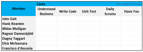
You can easily create such template in excel.
2. A More Robust Excel Timesheet Tracker
While the time sheet format shown in the above section is good, it is a wrong format if you need to analyze the timesheet entries of a 100 member project. Also in large projects usually members do few activities at a time. That means the above format (in section 1) will result in a sparse matrix.
Using a tracker log format is much more convenient to both record and analyze timesheet entries. Look at the example below:
![]()
We can use excel features like data validation drop downs, shared workbooks to make the timesheet entry and management a breeze.
3. Create a Resource Loading Chart – Project Management
Resource loading charts are a good way to show how busy the team members are in a project. At the outset the resource loading chart is nothing but a heatmap.
Look at an example resource loading chart below:

You can make a resource loading chart in MS Excel by following the below steps:
- The pre-condition for the resource loading chart is that we have clear data available to make one. This is where the robust timesheet tracker shown in section 2 of this post comes handy.
- First create a blank table in excel with team member names in first column and week numbers in first row. (Please note, you can make other types of resource loading charts by changing the Row and Column headers. For eg. You can show resource loading by Project and Team member)
- Assuming we have the time sheet data in the format shown in Section 2,
- Assuming “log_member_names” refers to the member name column and log_weeknum refers to the last column in the timesheet, we can write a simple COUNTIFS formula like this =COUNTIFS(log_member_names, “John Galt”, log_weeknums, 3)
- Once we calculate values for all team members using the above formula, we can apply conditional formatting to make the heat map. In Excel 2016 / 365, this is one step.

- That is all.
Download the Excel Timesheet & Resource Loading Chart Templates
You can download the excel time sheet template, timesheet tracker log template and resource loading chart template from here. Click the below links:
- If you have Excel 2016 / 365 or 2007 or above, download the .xlsx template
- If you have Excel 2003 and earlier, download the .xls template
- Download 24 Project Management Templates for Excel
What Next?
Timesheets are a great way to understand how the effort is spent. Even though project estimation models have become more and more effective, still lots of projects are overshooting budgets and timelines. And this is where timesheets can help you as a manager. While estimation looks in to future, timesheets look at past. Timesheets give feedback to your estimation models. This can help you in making better estimates in future.
In the next installment of this series, learn about tracking issues and risks using excel spreadsheets.
If you are new to the series, please read the first 3 parts as well.
- Preparing & tracking a project plan using Gantt Charts
- Team To Do Lists – Project Tracking Tools
- Project Status Reporting – Create a Timeline to display milestones
- While at it, also check out the bonus post about Burn Down Charts.
Resources for Project Managers
Check out my Project Management using Excel page for more resources and helpful information on project management.
Your thoughts and suggestions?
What are your ideas about timesheets using excel? Does your organization use excel as a way to manage timesheets or do you use some time tracking software? What is the granularity of detail captured in timesheets? As a project manager, what use do you find in time sheet data?
Share your ideas and experiences using comments.
*PS: If you are wondering what the heck TPS reports are, then you are spending way too much time with Excel buddy. And while at it, you missed the greatest comedy of all time. Go watch office space, now!
PPS: the TPS report image is from wikipedia.


23 Responses to “Learn Top 10 Excel Features”
What it looks like if excel without formula?? 🙂
It would be not excel it would just be fancy tables in which you could just use power point. (Chandoo) would Access be an alternative?
Awesome piece of work!!!
Great article.
Chandoo - my biggest interest in the article was the awesome word-graphic at the top - where did you go to get it done into a shape?
@Rich.. thank you. I used http://www.tagxedo.com/ to generate this word cloud. I took all the comments in the original post, pasted them in tagxedo website and set up the shape etc.
Awesome Chandoo.. You need always needs coffee to start up with. BTW , how did u created the Heart Shaped picture filled with High Repetitive text in it .. Please put it on your Next blog ...
Chandoo, good article. I’ve added a link to it from Connexion – our collection of the most useful and interesting spreadsheet-related articles from the web. See http://www.i-nth.com/resources/connexion
Hi,
Just one small question. Where the hell have been I in the past for not discovering this website sooner?
I've lost a job interview recently where even though I had the subject knowledge, I was not upto their mark in Excel.
Thank you for all the free tips, guidance and for creating this forum environment.
[PS: I've just been through the site for the 1st time, and have signed up for the newsletter. You can expect pretty stupid questions from me soon]
Hy Chandoo, you always inspire me with to explore something new in excel. This data structure table is only for excel 2007 or compatible to 2010. I recently installed latest excel version 2013 in my System and experience problems regarding operating according to previous one. I'm waiting your article relates to that excel version.
Thanks
Awesome article Mr. Chandoo and that is a awesome heart shaped pic you created. Great tips as well.
[...] Learn Top 10 Excel Features | Chandoo.org – Learn Microsoft Excel Online. [...]
Chandoo is awesome..
Thanks, i got better, And i always get 90.50 in my grade card but now i get 96.50 i improved because of the tutorials you gave, Thank You Very Much Chandoo Guy.
Hi chandoo, i am intersted in seeing the video or step by step done procedure of analysing the comments and presenting in the data percentage steps. I think this one would be first step in finding out how generally happens data calculation. Thank you.
As well i would like to know how to get that black shape art of your face which i see in chandoo. I am interested in making it for me.
Nice to see the features considered by Excel users to be most useful. It might be a good idea to also analyze StackOverflow Excel questions to see what keywords appear most often.
Here are my top 10 Excel Features (for advanced users):
http://www.analystcave.com/excel-10-top-excel-features/
Thanks a ton for this it totally helped with my homework ????
Very good effort
Thank you for this. Lots of learning in the links you've provided for this septuagenarian.
Pls send me new post
Dude, your humor ? ?
Loved your work.
Hello Sir,
I am Sanjeev Khakre and i from Indore City, India , I am your big follower and i have watch your videos and learnt a lots of excel trick or function and many more . thanks so much for all of your excellent support.
Your excel knowledge is real awesome.
Thanks
Sanjeev
Your work is excellent but pls willing to know more details about the features of microsoft excel
Chandoo Would Access be a better alternative than VB?