

For every column chart that is done right, there are a dozen that get messed up. That is why lets talk about 5 simple rules for making awesome column charts.
Tip: Same rules apply for bar charts too.
Rule #1: Start at zero
The first rule is simple. Always start your column charts at zero. When looking at column (or bar) charts, our mind measures height of each column and compares. So, if a column starts at some arbitrary point instead of zero, it can mess with our perception of how each column compares with other. Don’t believe me. See yourself.

Related: What is the most embarrassing charting mistake you made?
Rule #2: Thou shall sort
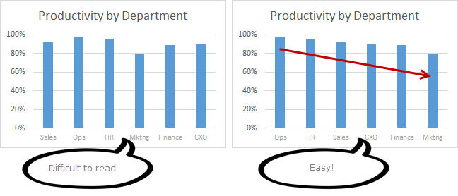
Sort your columns in a meaningful order. For example, sort them by descending order (of column heights), alphabetical order or chronological order. This will make reading the chart easy.
Rule #3: Slap a title on it
Give your chart a meaningful, clear title. Few examples of good and bad titles shown below.
 Rock star tip: Using smart titles & legends in your charts
Rule #4: Axis & Grid-lines vs. Labels
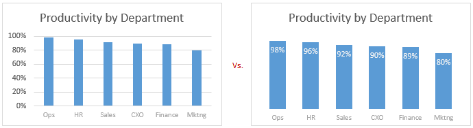
For most charts you can use data labels instead of axis & grid-lines. This will keep the chart clean.
If you choose to go with Axis and gridlines, then make sure they follow below guidelines.
- Axis label text should be relatively small & dull.
- Grid lines & axis line should be dull too.
- Do not display too many or too little major units on axis. You can change major unit size by selecting axis and pressing CTRL+1 (or axis options pane in Excel 2013).
Rule #5: Too much lipstick and you have a pig
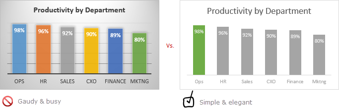
Make sure the formatting (colors, fonts, special effects, backgrounds etc.) of your chart are really subtle and meaningful. If you use too many colors, you end up with a pig. People will then focus on all these colors, fonts instead of actual data.
Few ways to add wow factor to your chart without messing it up:
- Highlight a particular column (for example max value, min value etc.) using different series technique.
- Use descriptive titles, clever data labels to show more information.
- Use drawing symbols or shapes to enhance the message of chart.
- Make your chart interactive to give users control.
- Add Emojis even
So there you go. Follow these rules and your column charts will stand tall.
Share your rules for making awesome column charts
While above rules capture the gist of making good looking column charts, there is more to learn and follow. So go ahead and share your rules and tips using comments. Teach us how you make stunning column charts (or bar charts). Post your comments below.
Make charts often? Check out these tips:
If your job involves analyzing & charting data, then check out below tips to learn more.


37 Responses
Re Rule #2: Alphabetic during should rarely if ever be used. It is arbitrary, and takes away meaning that is conveyed by a more meaningful sort order.
I guess if you are going to use a somewhat arbitrary sorting, alphabetic order at least means that you can quickly locate specific columns.
If you sort alphabetically for easier lookup, you’ve made a table.
If you want the data to be understood, it’s worth spending the time and mental effort to make it readable, and this post covers several ways to do that. Including sorting by an appropriate variable.
Apart from Sorting, the most important points which i liked is point no.3.
This gives a quick summary on analysis.
Regarding sorting orders – I generally have reports with more than one chart which relate to one another.
Because of this, I always make sure that whatever order the departments (or whatever I’m measuring) are sorted in the SAME order for each chart. Same thing goes for any colors I am using (if 2010 is red in chart one, it’s also red in chart two).
Good points. I do the same.
Rule #5 This is very true. ALWAYS remember your audience. 9/10 people in the room your presenting the charts to aren’t going to be savvy with excel, and the message you are trying to get conveyed will be distorted and in the worst case not heard.
Any sorting, Rule 2, has to be related to the context of the data and the story it is telling
Whenever I make a chart (not just a column chart, any chart), I always make the fill as ‘No fill’ and border as ‘No Border’ using the Format Chart option. Same with the Plot area of the chart using the Format Plot Area options. The default fill in chart and plot area is White. Visually on excel it does not make a difference, but if you were to paste the charts on a PPT, which i usually do, the white fill shows up as a faint border on the slide. Also making it transparent helps in handling on the PPT
Rule 4: Delete the % mark on the axis and add a subtitle “in percent”.
Rule 5 B: When using numbers above 1000 on the axis, just leave the zero’s and and x1000 above the axis. The bars.
In both cases: More space for the most important thing of the chart. The bars.
Rule #5
Hallo all,
for this is not problem prepare standards in every company (use TPM or other).
Example use colors in charts:
Yelow – last year (LY)
Blue – terget for this year
Red – results is bad compare to target
Orange – results is bad compare to target but better than LY
Green – results is good (compare to target and LY)
All people know this colors and you haven’t problem with presentation all KPI.
Pavel
Red and green are tough choices, since nearly 10% of the male population has some level of deficiency in distinguishing them.
Dear Jon,
i agree with you. Than is no problem for this people combine column asn line chart. Line is blue (target) column is act target (red&green). 10% male see only diff between column and line chart, 90% see color diff.
P.
If the columns are green and red, how can you say there’s no problem? Forget the colors, make the target hollow (bordeer only) and the actual filled.
Hey Jon, did the SUCCESS Concept arrive in US 😉
Joerg:
??
Actual = filled
Target = border only
… that one element (2.2.3) of Rolf Hichert Communication Concept
http://www.hichert.com/en/success/unify/114
Not in so many words (or by that acronym), but a lot has been written about these topics. Some of it is even good.
…use the bars from left to right for time issues and use it from top to bottom for structural issues like the example above.
That gives your reader a clear picture and he has not to start to think about the chart from scratch.
Also direct labeling instead of a legend is very helpful for line or stacked bar charts.
Colors are great but when making charts we often Forget blind color people. Idea for a contest ?
Otherwise great ideas as usual ! Thanks Chandoo !
We actually did have a color blind person on our management team – and for her (yes, it was a woman) – I used patterns instead of colors for fill.
For those who needed the colors (visual learners) – I used colors with the pattern.
So one range might be a blue cross-hatch, while another was a green dot. Another thing to keep in mind with color impairment is that some people cannot easily distinguish between shades of a color.
Basically – know your audience, and NEVER expect that the chart can speak for itself. Use labels and have numbers clearly visible in a graph nearby for reference by your users.
I have been using CVD-friendly color schemes a lot since a colorblind supervisor came to my facility (CVD = color vision deficiency). I got my color scheme from this website: http://jfly.iam.u-tokyo.ac.jp/color/
This is easy to learn creating awesome columns. Thanks a lot buddy.
I will use this in our excel sheets for sure. Keep updating! Cheers!
This is super super awesome! Thanks again chandoo, these are small thing, but makes a big difference when you actually want to depict the graphs to tell you entire story flawlessly. This is the best excel blog I have ever read and is simple yet on target.
Looking forward for many more similar easy to go tips.
Bhushan Sangle. Mumbai. India
I am not convinced that rule #1 is absolute. I report weekly on labor utilization (billable time/all time in period). It moves plus or minus about 5 percentage points. One half of a percent is significant.
However, on a bar chart starting at zero % the difference between say, 76.3% and 76.9% is nearly invisible.
In order to even see the small percentage % I start at a greater value than 0%. Is there a better way?
Line chart?
Or, if you have a target for labor utilization, you might be better served by charting % over/under target. (Although that chart too would be better as a line chart than a column.)
Crikey, my memory is bad. In fact we do use a line chart for the actual against a light colored area chart for the goal. the vertical axis begins at about 60%.
Another awesome post. Its really amazing to see you run this whole blog around Excel. There is always so much to explore.
Sorting charts is usually a bad idea unless you have error bars or a time series. I can take random data, sort the groups, and hey presto it looks like there is a descending pattern to the data.
On Data labels (see #4 as sample), is there an easy (and nice) way where I can add on additional data labels below the X axis?
For example, I would like to show the sample size for each department. So, it is like an additional row below the Department Row (X-axis).
I know i can use text boxes for this, but i have problems aligning all the text bosses so it will look neat.
Any tips?
Cyndi –
Include it in your category labels (the X axis labels). So instead of “Ops”, “HR”, “Sales”, etc, enter “Ops50”, “HR42″, Sales37”, etc. into the cells, where is a line feed, which you get by holding Alt while pressing Return.
For hottest information you have to pay a quick visit the web and on the web I found
this website as a best site for latest updates.
Great post about column charts and this is useful information, thanks
keep sharing