Often when we are making spreadsheets for forecasting or planning we would like to keep the starting month dynamic so that rest of the months in the plan can automatically rolled. Don’t understand? See this example:

This type of setup is quite useful as it lets us change the starting month very easily. We can use such a set up in, for eg. Gantt Charts to change the project start dates with ease. Today we are going to learn how to set up automatic rolling months in Excel.
To set up such dynamic rolling months in Excel, just follow these simple steps:
1: Create a list of all the months
Enter the month names in a bunch of cells (Tip: Just enter the first month name and then click at the bottom right corner of that cell and drag to get all the other month names). Let us call this range as B5:B16. If you prefer, name this range as “lstMonths“.
2: Set up data validation drop down list on the first cell for automatic rolling
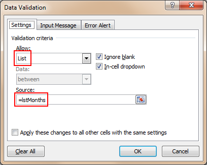
Now, let us assume we will use cells A1:A12 for automatic rolling months. Select A1 and set up data validation list on it (so that users can only enter a valid month in that cell) and use “List” type as validation. See below:

3: Now write formulas so that we fetch consecutive months based on first month
(Thanks to comments from Jeff, Hui, Vipul and others. I found a simpler and easier way to write the formula)
We will simply use Excel’s date formulas so that we can fetch consecutive rolling months based on the first selection.
Assuming the date is selected in cell A1,
In A2, write the formula:
=DATE(2010,MATCH($A$1,lstMonths,0)+COLUMNS($A$2:A2),1)
What is above formula doing?
- It is using the DATE Formula to create a next months first date.
- The part MATCH($A$1,lstMonths,0) is used to fetch the position of selected month in the range lstMonths
- The part COLUMNS($A$2:A2) is used to generate the sequential numbers in excel.
- Make sure you have formatted the cells A2:A12 as “date” with code “mmm” to show 3 letter month codes.
- Rest all you can figure out easily 🙂
A more complex solution
in-case you got some other types of values instead of months:
To make it a bit simple, I will use a helper cell where we can identify the position of selected month in the list of months, like this:

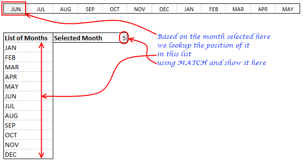
I have assumed that Jan is 0, Feb is 1 … Dec is 11. Also, assume, the helper cell is in $B$4.
Now, If the selected month is “5”, then the other months will be 6,7,8,9,10,11,0,1,2,3,4.

The interesting part here is the sudden jump from 11 to 0 as highlighted above.
To get this type of output we must use an excel formula called as MOD.
What is Excel MOD Formula?
MOD formula takes 2 numbers tells us the remainder when first number is divided by second number. [Excel MOD formula, Introduction, Syntax & Examples]
So how to use MOD formula to setup rolling months?
Very simple. We just take the value in $B$4 (position of the first month in the list) and then add +1 to it and then find out the MOD of it when divided by 12. We now use this number to fetch the corresponding month from lstMonths.
We use +2 for second month…. +11 for the last month.
We can simplify the +1, +2..+11 part by using COLUMNS formula to generate the sequential numbers for us.
The formula looks like this:
=INDEX(lstMonths,MOD($B$4+COLUMNS($A$2:A2),12)+1)
- The Mod portion of this formula tells the position of the second, third, fourth, … eleventh month based on the first month.
- We have to add +1 to output from MOD because we are using 0,1,2,3 positioning the month in B4, where as INDEX use 1,2,3,4 positioning.
- INDEX formula then fetches the corresponding month from lstMonths(orB5:B16)
That is all.
Download the example workbook and learn on your own
I have prepared a short example workbook where this technique is demonstrated. Feel free to download it and play with it to learn more.
Where would you use such a rolling month setup?
I have once used the rolling month set up in a forecasting spreadsheet (where we made cash flow projections for a startup we were planning to acquire). I am also planning to upgrade my gantt chart templates include rolling month setup.
What about you? Where would you use automatic rolling months?


14 Responses to “How many ‘Friday the 13th’s are in this year? [Formula fun + challenge]”
in C3=2016
in C4=3
in C5=1 (the first next year with three Friday the 13ths)
=SMALL(IF(MMULT(--(MOD(DATE(C3+ROW(1:1000),COLUMN(A:L),13),7)=6),ROW(1:12)^0)=C4,C3+ROW(1:1000)),C5)
formula check in the next 1000 years
This will generate a table of counts of Friday the 13th's by year. If I didn't screw it up the next year with three is 2026.
I created a simple parameter table with a start date and end date that I wanted to evaluate. That calculates the number of days and generates a list of those days. Then filter and group. The generation of the list in power query (i.e. without populating a date table in excel) is pretty cool, otherwise this isn't really doing anything than creating a big date and filtering/counting.
let
Source = List.Dates(StartDateAsDate, Days2, #duration(1,0,0,0)),
ConvertDateListToTable = Table.FromList(Source, Splitter.SplitByNothing(), null, null, ExtraValues.Error),
AddDayOfMonthColumn = Table.AddColumn(ConvertDateListToTable, "DayOfMonth", each Date.Day([Column1])),
AddYearColumn = Table.AddColumn(AddDayOfMonthColumn, "Year", each Date.Year([Column1])),
AddDayOfWeekColumn = Table.AddColumn(AddYearColumn, "Day of Week", each Date.DayOfWeek([Column1])),
FilterFriday13 = Table.SelectRows(AddDayOfWeekColumn, each ([DayOfMonth] = 13) and ([Day of Week] = 5)),
Friday13thsByYear = Table.Group(FilterFriday13, {"Year"}, {{"Number of Friday the 13ths!", each Table.RowCount(_), type number}})
in
Friday13thsByYear
With the parameters replaced by values should you want to play along at home. This runs for 20 years starting on 1/1/2016.
let
Source = List.Dates(#date(2016,1,1), 7300, #duration(1,0,0,0)),
ConvertDateListToTable = Table.FromList(Source, Splitter.SplitByNothing(), null, null, ExtraValues.Error),
AddDayOfMonthColumn = Table.AddColumn(ConvertDateListToTable, "DayOfMonth", each Date.Day([Column1])),
AddYearColumn = Table.AddColumn(AddDayOfMonthColumn, "Year", each Date.Year([Column1])),
AddDayOfWeekColumn = Table.AddColumn(AddYearColumn, "Day of Week", each Date.DayOfWeek([Column1])),
FilterFriday13 = Table.SelectRows(AddDayOfWeekColumn, each ([DayOfMonth] = 13) and ([Day of Week] = 5)),
Friday13thsByYear = Table.Group(FilterFriday13, {"Year"}, {{"Number of Friday the 13ths!", each Table.RowCount(_), type number}})
in
Friday13thsByYear
=MATCH(3,MMULT(N(WEEKDAY(DATE(C3+ROW(1:100)-1,COLUMN(A:L),13))=6),1^ROW(1:12)),)+C3-1
It should be pointed out that Alex's solution, unlike some others, has the additional advantage of being non-array. My solution was nearly identical but with -- and SIGN instead of N and 1^.
=C3-1+MATCH(3,MMULT(--(WEEKDAY(DATE(C3-1+ROW(1:25),COLUMN(A:L),13))=6),SIGN(ROW(1:12))),0)
Sub Friday13()
Dim StartDate As Date
Dim EndDate As Date
Dim x As Long
Dim r As Long
Range("C7:C12").ClearContents
StartDate = CDate("01/01/" & Range("C3"))
EndDate = CDate("31/12/" & Range("C3"))
r = 7
For x = StartDate To EndDate
If Day(x) = 13 And Weekday(x, vbMonday) = 5 Then
Cells(r, 3) = Month(x)
r = r + 1
End If
Next
End Sub
Calculate next year with 3 Friday 13th. Good for 100 years different from year entered in cell C3
Sub ThreeFriday13()
Dim StartDate As Date
Dim EndDate As Date
Dim x As Long
Dim WhatYear As Integer
Dim Counter As Integer
Range("E7").ClearContents
StartDate = CDate("01/01/" & Range("C3") + 1)
EndDate = CDate("31/12/" & Range("C3") + 100)
Counter = 0
For x = StartDate To EndDate
If WhatYear Year(x) Then
WhatYear = Year(x)
'Different year so reset counter
Counter = 0
End If
If Day(x) = 13 And Weekday(x, vbMonday) = 5 Then
Counter = Counter + 1
If Counter = 3 Then
WhatYear = Year(x)
Exit For
End If
End If
Next
Range("E7") = WhatYear
End Sub
*RE-POST as not equal did not show earliuer
Calculate next year with 3 Friday 13th. Good for 100 years different from year entered in cell C3
Sub ThreeFriday13()
Dim StartDate As Date
Dim EndDate As Date
Dim x As Long
Dim WhatYear As Integer
Dim Counter As Integer
Range("E7").ClearContents
StartDate = CDate("01/01/" & Range("C3") + 1)
EndDate = CDate("31/12/" & Range("C3") + 100)
Counter = 0
For x = StartDate To EndDate
If WhatYear NE Year(x) Then
WhatYear = Year(x)
'Different year so reset counter
Counter = 0
End If
If Day(x) = 13 And Weekday(x, vbMonday) = 5 Then
Counter = Counter + 1
If Counter = 3 Then
WhatYear = Year(x)
Exit For
End If
End If
Next
Range("E7") = WhatYear
End Sub
earlier*
I've a doubt with using array formula here.
In sample workbook, I tried to replicate the formula again.
=IFERROR(SMALL(IF(WEEKDAY(DATE($C$3,ROW($A$1:$A$12),13))=6,ROW($A$1:$A$12)),$B7),"")
For this I selected C7 to C12, and typed the same formula and pressed ctrl+alt+Enter. But in all cells it is taking $B7 (and not $B7, $B8, $B9.... etc)
and since it is array formula I can't edit individual cell.
Please guide.
Thanks
Hi Chandoo,
Cool stuff. You need to clarify that the answer of 5 represents the 1st month in the year that has a Friday the 13th, and not the number of Fridays the 13th in the year. Subtle, but important difference.
Thanks,
Pablo
I like the MMULT() function far more, but here's how I would have tackled it. It uses an EDATE() base and MODE() over 100 years. I'm assuming that 100 years is enough time to catch the next year with 3 friday 13th's. Array entered, of course.
{=MODE(IFERROR(YEAR(IF((WEEKDAY(EDATE(DATE(C3, 1, 13), ROW(INDIRECT("1:1200"))))=6), EDATE(DATE(C3, 1, 13), ROW(INDIRECT("1:1200"))), "")), ""))}
Finding all the Friday the 13ths in a Year:
=SUMPRODUCT((DAY(ROW(INDIRECT(DATE(C3,1,1)&":"&DATE(C3,12,31))))=13)*(TEXT(ROW(INDIRECT(DATE(C3,1,1)&":"&DATE(C3,12,31))),"ddd")="Fri"))
{=sum(if(day.of.week(DATe($YEAR;{1;2;3;4;5;6;7;8;9;10;11;12};13);1)=6;1;0))}
just list the years