
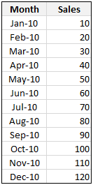
Here is a problem we face very frequently. You have a list of values by months. And you want to find out the totals by Quarter. How do you go about it?
There are 2 options:
- You can make a pivot report from the data and then group dates in that to find totals by quarter
- You can write formulas to find the totals by quarter
While option 1 is good for knowing the values, we need option 2 if you want the values to be fed to another report, chart or dashboard.
Writing Formulas to Get Quarterly Totals from Monthly Data:
First, understand a little math formula called ROUNDUP():
ROUNDUP formula takes a number and rounds it up to the nearest fraction as specified by you. So for eg.,
ROUNDUP(1.234,1) = 1.3ROUNDUP(1.234,2) = 1.24ROUNDUP(1.234,0) = 2ROUNDUP(1.0,0) = 1
Now, assuming your monthly data is in cells B4:C15,
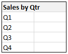
Our objective is to find Quarters from dates and then add up all items in Q1 against Quarter 1.
We can get the month from a date using MONTH() formula. If we divide the month by 3 and then round the value up to nearest integer we will get the Quarter.
So, A formula like =ROUNDUP(MONTH(B4)/3,0) should tell us the quarter for the month in the cell B4.
So the final formula for calculating sum of all the sales in Q1 is =SUMPRODUCT((ROUNDUP(MONTH(B4:B15)/3,0)=1)*(C4:C15)).
How this formula works?
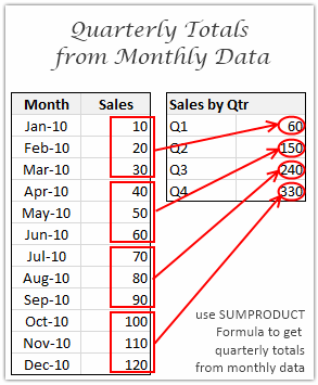
Well, the portion ROUNDUP(MONTH(B4:B15)/3,0)=1 gives a bunch of 1 and 0s, one where the month belongs to Q1 and zero where it is not. When you multiply these ones and zeros with actual sales values in C4:C15, you get the total sales in Q1.
Since SUMPRODUCT has magical powers, it just processes all these ranges of data without batting an eyelid.
Download the example worksheet and play with this formula
Go ahead and download the example workbook and play with SUMPRODUCT formula to understand this better.
How do you calculate Quarterly Totals from Monthly Data?
Do you know a better way to do such calculation? How do you usually do it? Please share your tricks and ideas using comments.


34 Responses
Chandoo,
Very nice post. In most cases I would use a formula such as yours so that copying is automatic. But for instructional purposes, consider this alternative for the Q1:
=SUMPRODUCT((MONTH(B$4:B$15)={1,2,3})*C$4:C$15)
Besides being shorter, this formula is crystal clear in function. Then for the other quarters you would just change the array constants to the months of that quarter. For example, Q2:
=SUMPRODUCT((MONTH(B$4:B$15)={4,5,6})*C$4:C$15)
Now I know there are a lot of accountant types out there that think using constants in a formula is some sort of heresy. I think that idea is silly. If the formula is clear and maintainable, constants are ok by me. But if this idea shakes anyones soul, these constants could easily be encapsulated in named formulas and then the formula above could look like this:
=SUMPRODUCT((MONTH(B$4:B$15)=Quarter1)*C$4:C$15)
The SUMPRODUCT function is truly magical, as you put it. This article goes into some advanced uses:
http://www.excelhero.com/blog/2010/01/the-venerable-sumproduct.html
Regards,
Daniel Ferry
excelhero.com
I have a column of dates(xx/xx/xx) on a sheet that represents when a task is completed. How do I code a formula on a separate sheet(Summary Page) of the total number of completions within a quarter?
ie;
Task Date Completed
task1 02/05/14
task2 04/01/14
task3 08/01/14
I need a formula that scans that column and then adds the number of tasks completed within each quarter of the year.
Chandoo,
as usual, great tip.
Ever since i read this post, I am struggling with a table that has the same layout as the example, and I wanted to add the totals per year and per Q, years as rows, Qs as columns. The first thing I’ve noticed is that I had to add the double minus to the roundup portion in order to make it work, even my dates ARE dates…but what i cannot figure out is how to summarize by year. I’ve tried adding a Year(a1:a20)=2010 to the sumproduct, but it returns 0, and I have the Pivot table below to prove that wrong (aaah, how easy was to have that with the pivot table….!!)
btw, I was playing around with PTs, adding calculated fields and items to solve variations between Actuals and Budgets and Prior Years. Once you get the formulae right, it’s sooooo easy to do, and the results are awesome !!!
all the best,
Martín
Amended Chandoo’s formula to add a year and it worked fine.
SUMPRODUCT((YEAR($B$4:$B$15)=2010)*(ROUNDUP(MONTH($B$4:$B$15)/3,0)=ROWS($E$4:F4))*$C$4:$C$15)
Chandoo
I generally do quarters in the same way galthough I would have changed the number format of cells E4:E7 to Q0, so that I could reduce to formula length by referring directly to these cells. SUMPRODUCT((ROUNDUP(MONTH($B$4:$B$15)/3,0)=E4)*$C$4:$C$15).
I like Daniel’s suggestion of a named range. Great site.
Thanks Chandoo,
I use a tbl to create relationshipp for each period to its quartile
Jan Q1
Feb Q1
Mar Q1
Create a lookup in a helper column to lookup the correct quartile.
Use Sumif on the column with the quartile
Best regards,
Winston
@Daniel: Excellent insights as always. I am finding SUMPRODUCT formula really really powerful.
I didnt know that we can write conditions like ={1,2,3}. I remember trying that but it didnt work. thanks for telling me how to do it. I like your idea of named ranges. It will keep things simple and also let the reports to easily transformed if one needs to change Q1 from JAN-MAR to APR-JUN.
@Martin: See Alan’s comments. Also, I liked your question, so I am doing a follow up post on it today. Refer to it to find out how you can get quarterly totals from multi-year monthly data.
@Alan: Very good tips. Thank you. Infact, in the download file you would find the formula to be slightly different. I used ROWS() so that I need not change the values for each quarter. I guess either technique works fine.
@Winston: Thanks for sharing your technique. Using helper columns is a fine option too. It keeps the formulas clean and simple. I was just curious and investigated to find if there is a formula that would avoid helper columns.
Chandoo, I learn so much from your posts. Thank you for this!
I was wondering, how would this get applied to a dashboard with a dynamic date slider?
Right now I show sales for the week, month, and year based on the date I choose. I’ve yet to discover how to calculate quarterly numbers based on my date selection.
My date is determined by: =DATE(2018,12,31)+7*(A2-1) with A2 updating based on the slider.
Sales This Month is calculated as: =SUMPRODUCT((MONTH(Data[Order Date])=MONTH(D2))*(Data[Sales Amount])) with D2 containing the date formula above.
ANy suggestions?
Thanks for your question Jason.
It seems you have data at date (or even lower level). In such cases, you need either two conditions or probably SUMIFS to solve this. For example with SUMIFS,
=SUMIFS(data[sales amount], data[order date],”>=”&quarter_start, data[order date],”<"&quarter_end) where quarter_start = date(year(a2), choose(month(a2), 1,1,1,4,4,4,7,7,7,10,10,10), 1) and quarter_end = date(year(a2), choose(month(a2), 4,4,4,7,7,7,10,10,10,13,13,13), 1) can work.
How about if we have the data in weeks and we want to roll it up in Q1, Q2, Q3, Q4
will this work for Q1:
=SUMPRODUCT((MONTH(B$4:B$15)={1,2,3,4,5,6,7,8,9,10,11,12,13})*C$4:C$56)
nice article to use the new things on the excel to calculate the needed ports…The use of tables shows the image view than the wordings, since images are easily recorded in the mind of users than the words to be read…
I have an issue, much different yet has some similarities…
I have two worksheets… ‘Summary’ worksheet and ‘Stop pays’ worksheet.
The summary sheet has the $ amount of checks paid each week. (example. A1= 1/1/10, B1= $100,000.00; A2= 1/8/10, B2= $120,000.00, A3= 1/15/10, etc…for 52 weeks)
On the stop pays sheet is a list format of each check that was voided at a later date… (example. column A= original check date, column B= check voided amount, column C= void date. A2= 1/1/10, B2= -$100.00; A3 = 1/1/10, B3= -$150.00; A4= 1/1/10, B4= -50.00; etc…)
On the summary sheet in C1, I need to calculate the total checks actually paid out. I have been trying to use combinations of SUMPRODUCT with VLOOKUPS, but can’t get anything to work. The result in C1 should $99,700.00
Any thoughts, all help is appreciated. Thanks, Kyle
@Kyle
Give this a try in Summary!C1 and copy down
=SUM($B$1:B1)+SUMPRODUCT(1*(‘Stop Pays’!A2:A100<=Summary!A1)*('Stop Pays'!$B$2:$B$100))
@Kyle… you can use sumif formula…
Assuming your summary sheet is in range A1:B10, stop pays sheet is in range A1:B20.
in summary c1 write = b1 – sumif(‘stop pays’!$a$1:$a$20,a1,’stop pays’!$b$1:$b$20)
Read more about sumif formula here: http://chandoo.org/wp/2008/11/12/using-countif-sumif-excel-help/
@Hui. Thanks, but for some reason this only worked for the first row (C1), when I copied down the results werent accurate.
@Chandoo. This seems to work perfectly. Thank you.
Thanks again.
@ Kyle
Chandoo’s formula is giving the amount each month (Cheques – Stop Pays)
Mine is giving a running total from 1/1/10 to the date in Summary!Column A
I have monthly data in one sheet and want to calculate quarterly and annual data is two other sheets. all monthly data is arranged across columns. so A1 is jan 2000, b1 is feb 2000, c1 is march 2000 and so on.
Please help
@Priyank: Assuming your months are (in date format) in A1:X1 and corresponding values are in A2:X2, you can calculate quarterly totals like this:
=SUMPRODUCT((ROUNDUP(MONTH(A1:X1)/3,0)=1)*(A2:X2)) for Q1. Modify it to get Q2… etc.
you can use similar logic with YEAR() to get yearly totals.
This formula is not working properly in one of my sheets with horizontal cash flows using columns instead of rows. For example, Q1 only sums M1 and Q2 is summing up M2:M4. It doesn align propoerly. The formula works if I create a simple test using same format in excel but not in the model. Can I send the excel to someone?
Thanks,
Marc
Item 01-Mar 02-Mar 03-Mar 04-Mar Tot.
Soap 24 12 15 13 (E5-F5)+(G5-F5)+(G5-H5)
Ketchup 12 10 8 14
Tea 10 8 5 8
Soup 12 7 9 11
Coffee 22 26 14 13
Hi!!,
I need your help in fixing above problem.
I do get day day wise closing stock of my company.To get day sales have to
substract today’s no from prev.day’s no. But sometimes today’s no is big due to receipt of stock.That time I need to substract prev.day’s no from today’no. Pls see formula in tot column.Like this I have to do for 31 days and 250 items.I want one formula in one cell give final result(tot)by satisfying above conditions else I have to punch a formula in above column which is boring ang time consuming.Thanks in advance.
Hi Chandoo et al,
My question builds on the post regarding quarterly totals from monthly data. I’m having trouble getting the formula to work when the time period I want quarterly totals for exceeds 12 months. In my case, I have 240 months and need these to be collapsed into 60 quarters. Any suggestions? Or should I simply cut and paste the formula for each 12 month period?
thanks
Hi Chandoo,
I have a similar problem, but with a twist. I often compare actual and budget data where the actuals are in one range with Jan-Dec data and the budget is another range with Jan-Dec data.
The problem I have is that at the beginning of the year I know the budget for all 12 months, so my range is populated for Jan-Dec. The actual data is populated as we complete those months.
Here’s the rub: when caluclating totals for Oct, say, the formula to retrieve Q4 data needs to be smart enough to NOT include the November and December budget amounts, which are already populated in the table.
how can I do the same using SQL query?plz help
How do we use this for getting totals for the latest qtr? anybody?
My challenge is I don’t want to use a helper column. Want to derive the latest qtr and then average the numbers for that qtr . Ex this gives an error :
AVERAGEIF((ROUNDUP(MONTH($A$2:$A$7)/3,0),(ROUNDUP(MONTH(MAX($A$2:$A$7))/3,0)),B2:B7))
Hi
I am arranging a spread sheet for work but am struggling with a date function. we have customers in our service for up to 2 yrs, however we have to calcuate the number of days they have been in service each quarter. For example Q1 will run from 15/01/15 to 06/04/15 but my customer could have joined on 03/09/14 … i don’t want to calulate all the days just the days in the quarter… which should be upto 91 days max. Can any one help at all?
Dear all
I can see your formula and I think it works perfectly for what I want to achieve, ie pull quarterly figures from a range showing monthly data. There’s only one problem. I cannot follow how the sumproduct formula is working in this case. Could anyone please help with an explanation on what is going on in that formula so I can hopefully be able to apply it.
Thanks
Hi,
I need to come up with a way to show the current quarters info, this would be run off the month end date.
For example: If the month end date is 28.2 then I need to bring back Jan data and Feb data or if the end date was 31.3 I would need to total Jan, Feb and Mar data.
I am thinking of creating unique references such as the quarter plus which month it is in the quarter ie if it was feb, the unique reference would be Q12 (Q1 for the quarter and 2 for the month as it is the 2nd month in the quarter). Would I need to use an index or offset formulae………
Any help would be appreciated.
Greetings,
Can we make this a little more involved just month and sales results.
What if I have the following columns:
Vendor Name
Market
Line of Business
Month
Sales
Now I want to calculate the average quarterly sales by vendor, Market, and Line of Business
Hello Hesham… thanks for your question. You should use Pivot Tables for such things. See here for a getting started guide – https://chandoo.org/wp/excel-pivot-tables-tutorial/
Im a little confused, I have the following table of sales
Sales Sheet
ColA=dates(dd/mm/yyyy)
ColE=amount(total amount of sales in $)
eg
A E
11/02/2020 $20.00
01/01/2020 $15.00
03/12/2020 $16.00
05/07/2020 $23.00
etc etc
Report Sheet
I want to report the running total of sales for each quarter and update the figures here as more get added
Cell B2= Quarter1 total
Cell B5= Quarter2 total
Cell B8= Quarter3 total
Cell B11= Quarter4 total
How do I read the Sales Sheet column A selecting all dates for each quarter and sum total them in The Report sheet. I have tried mucking about with your formula but I just keep getting errors, any help much appreciated
I have problem Statement, my data are monthly i need to do comparison at QTD level say i am second quarter May (so my data should only pick April and May total) and( when in June it should pick Apr+ May +June) – can i your help on this
Jan Feb Mar Apr May Jun Jul Aug Sep Oct Nov Dec
1 2 3 4 5 6 7 8 9 10 11 12