
Excel Paste Special is one of my favorite features. So I was naturally thrilled when I discovered that you can use paste special to paste formatting from one chart to another.
When we have multiple charts, ensuring consistent color schemes, fonts etc. is very important. Often we individually format the charts because they have different chart types or source data. But instead, you can just use paste special to copy and paste chart formatting (formatting of labels, grid line settings, axis settings, colors, legends, titles) from one chart to another. See this small tutorial.
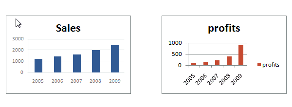
- To do this, Select the source chart, press Copy (or CTRL+C), now select the destination chart, go to Paste Special (or press ALT+ES). From the dialog select “Formats”.


