
Situation
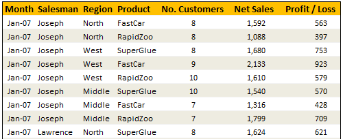
Not always we want to lookup values based on one search parameter. For eg. Imagine you have data like below and you want to find how much sales Joseph made in January 2007 in North region for product “Fast car”?
Data:
Solution
Simple, use your index finger to scan the list and find the match 😉
Of course, that wouldn’t be scalable. Plus, you may want to put your index finger to better use, like typing . So, lets come up with some formulas that do this for us.
You can extract items from a table that match multiple criteria in multiple ways. See the examples to understand the techniques:
| Using SUMIFS Formula [help] | |
| Formula | =SUMIFS(lstSales, lstSalesman,valSalesman, lstMonths,valMonth, lstRegion,valRegion, lstProduct,valProduct) |
| Result | 1592 |
| Using SUMPRODUCT Formula [help] | |
| Formula | =SUMPRODUCT(lstSales,(lstSalesman=valSalesman)*(lstMonths=valMonth)*(lstRegion=valRegion)* (lstProduct=valProduct)) |
| Result | 1592 |
| Using INDEX & Match Formulas (Array Formula) [help] | |
| Formula | {=INDEX(lstSales,MATCH(valSalesman&valMonth&valRegion&valProduct, lstSalesman&lstMonths&lstRegion&lstProduct,0))} |
| Result | 1592 |
| Using VLOOKUP Formula [help] | |
| Formula | =VLOOKUP(valMonth&valSalesman&valRegion&valProduct,tblData2,7,FALSE) |
| Result | 1592 |
| Conditions: | A helper column that concatenates month, salesman, region & product in the left most column of tblData2 |
| Using SUM (Array Formula) [help] | |
| Formula | {=SUM(lstSales*(lstSalesman=valSalesman)*(lstMonths=valMonth)* (lstRegion=valRegion)*(lstProduct=valProduct))} |
| Result | 1592 |
Sample File
Download Example File – Looking up Based on More than One Value
Go ahead and download the file. It also has some homework for you to practice these formula tricks.
Also checkout the examples Vinod has prepared.
Special Thanks to
Rohit1409, dan l, John, Godzilla, Vinod
Similar Tips
- Excel SUMIFS Formula – What is it, how to use it & examples
- Excel SUMPRODUCT Formula – What is it, how to use it & examples


11 Responses to “Use Alt+Enter to get multiple lines in a cell [spreadcheats]”
@Chandoo:
One more useful trick.......
In a column you have no. of data in rows and need to copy in the next row from the previous row, no need to go for the previous rows but entering Alt + down arrow, you will get the list of data, (in asending order), entered in the previous rows...
This is another great tip. I use this all the time to make sense of some *very* long formulas. As soon as the formula is debugged I remove the break.
Great tip Chandoo!
I use this feature often and it has even gotten the, "how did you do that" response.
Thanks!
@Ketan: Alt+down arrow is an awesome tip. I never knew it and now I am using it everyday.
@Jorge, Tony: Agree... 🙂
[...] Day 1: Insert Line Breaks in a Cell [...]
how can we merge a two sheet.
excellent idea. Chandoo you are genious
Hi chandoo,
I have used ctrl+enter to break the cell. But I did not get the result.
Please tell me how can i break the cell in multiple lines.
Hi, Ranveer,
Its not Ctrl+enter to break the cell, use Alt+Enter to make it happen.
hi Chandoo....
how we can use Alt+Enter in multiple rows at the same time please reply hurry i have lot of work and have no time and i m stuck in this. 🙁
Alt+J worked once 🙁
So I found another more reliable way:
=SUBSTITUTE(A2,CHAR(13),"")
Where A2 is the cell that contains the line breaks which the code for it is CHAR(13). It will replace it with whatever inside the ""