

Do you know that in Excel 2010 you can create your own Ribbon tabs and add anything to them, including your own macros? Today, we are going to take a look at this useful feature and learn how to add your own macros as buttons to Excel Ribbon.
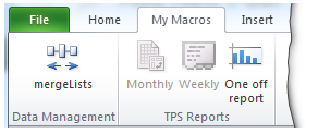
Steps to Add your own macros to Excel Ribbon [Excel 2010]
Step 1: Go to Excel Options to create a new ribbon
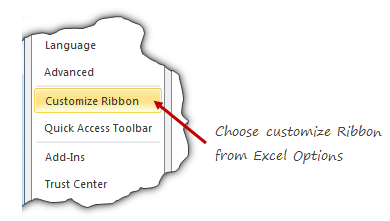
The first step is simple. Click on File menu and go to Excel Options. From here, click on Customize Ribbon.
Step 2: Add a Ribbon for your macros, Add your macros
This step is even simpler. Just create a new tab, add new groups as needed and add your macros. To add macros,
- Choose macros from the leftside area, then select all your personal macros and add them to your own ribbon.
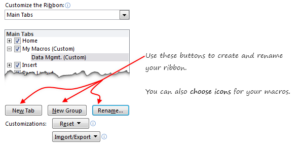
Bonus tip: You can also change or set icons for your macros. So that they look awesome on your new ribbon.
Step 3: Click ok and be done!
Really there is no step 3. Just click ok and play with your new ribbon.
Things to keep in mind while creating new ribbons
With Excel 2010, Microsoft introduced the capability to create and customize ribbon. While this is a powerful feature, it does have some gotchas. Keep these in mind while adding new ribbons or customizing existing ones.
- When you add a group or tab, excel doesn’t ask you for a name. Make sure you click on “rename” button to change the name to something you remember.
- You cannot add commands to an existing excel defined group. You can however add groups to existing ribbons.
- The ribbon and QAT customizations you do are local to your installation of excel only.
- However, you can export the customizations and import them to other computers.
Do you use Customized Ribbons in your Excel?
Even though this is a very powerful feature, I have not used it much as most of what I do is found on regular ribbons. However, for those of you frequently accessing a set of features, you can add all of these (and any personal macros) to a custom ribbon and get rid of everything else. It looks clean and saves a lot of mouse travel.
What about you? Do you use customized ribbons? Have added macros to them? Please share your experience using comments.
Add VBA & Macros to your Skills Ribbon
Do you know that you can join our online VBA Classes and learn how to create powerful macros from scratch? Our online VBA Class is a step by step program aimed to teach you all the basics and advanced macro programming so that you can save time, look awesome and get things done faster. Click here to join us today.
References to Learn More
Ribbon & Quick Access Toolbar help us find what we want and do. That said, they are not the easiest interfaces for those of us migrating from menus & t0olbar world (read Excel 2003 or earlier). Do not worry, we have a lot of helpful material on these topics. Check out,


14 Responses
Can this be done in 2007?
@Bob… Not without some sort of VBA / Add-in. However, you can add macros to QAT in Excel 2007. The process is similar. See the link in References section for more.
I’ve created a custom ribbon for a couple of useful macros, including one which copies data to the clipboard in a certain format for use with a third party reporting program, and another which saves text files using ‘unsual’ delimiters, again for use with third party programs.
I’ve also used a Custom UI Editor and VBA to create an Add-In which adds a bespoke menu and commands to Excel for use by a whole department which enables them to quickly and easily access useful files, tools and formatting macros etc – and these menus look so much nicer than the old Excel 2003 ones!!
Thank you for this description, it helped me wonderful .. (finally) now, we are on the office 2010 – world
Hi Chandoo,
Do you know if there is any way to use anything other than the default set of icons that Microsoft provide? Some of them don’t scale very well and come out pixelated. Also, sometimes I struggle to find an icon that really represents what the macro does.
Is there any way I can import my own pngs as icons?
Thanks
Jason
I have successfully set up a custom ribbon with macros in a PERONAL.XSLB file. When I copy this file to other computers and import the exported UI file I get a message that the macros are not available. What I have discovered is that the location of the Macros still references the original computer in the ribbon.
I was afraid that my only solution was to modify each ribbon until I found an answer on: http://datapigtechnologies.com/blog/index.php/excel-2010-customizable-ribbon/ Kathleen supplied the answer.
HI,
I have a problem whereby I have created some marcos, made a custom ribbon and now have buttons which nicely run the marcos. However, if I move the location of the excel then it does not work anymore.
What do I need to do to make it work?
Thanks,
The customize ribbon feature is great but I realized it must be used with care, especially in a client environment, because any changes are global to the Excel installation. Maybe there is a way around this that I am not familiar with. For example, I may add a macro and a corresponding icon that is used by one person in a work group. Other users will see the icon but not have access to the macro.
Great exp,./ please help me to create a ribbon in Excel 2007, as in 2010 there are two options like creating ribbon for tool bar and customize quick access toolbar, but in 2007 there is only option of Quick access, so guide me how to create Customize the ribbon in 2007
Hi
Above tip talks about adding new tab or creating a new gropu in ribbon. How add an icon in that tab and assign macro to it.
Thanks,
Asheesh
Well, of course this doesn’t really work. It used to be so easy – back ten years ago before Microsoft started hiring idiots. Anyway, now the “macro” option is completely blank. Nada. Zip, Leetho. Nothing to add – pretty button nor ugly button.
I’ve created a macros ribbon, but it is only showing icons for the 36 macros!
How do I get the list to show the macro names please?