
Update: Check out the results at Budget vs. Actual Charts
Here is your chance to get a copy of The Visual Display of Quantitative Information by Edward Tufte. Interested ? Read on,
Reader Sumit writes in to ask,
I am working on creating a visualization for data attached in the excel file (see below). Since I was not sure as to what would be the best way in which this data can be presented, I thought I will ask for your assistance.
Would it be possible for you to play around with the data and share your ideas as to the best possible way to represent this data graphically.
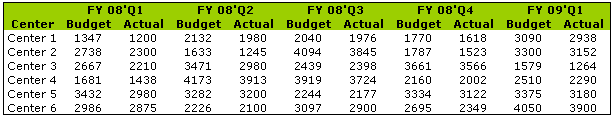
Download the data in a CSV file
Even though I have few ideas on visualizing budget vs. actual performance, I thought this is a great way for You, my dear reader, to share your ideas.
So what are you waiting for? Go ahead and tell us how you will visualize this data. The best visualization maker will get eternal glory and a copy of The Visual Display of Quantitative Information by Edward Tufte.
Go!
For inspiration and ideas visit: Stacked Bar chart techniques, 14 ways to visualize last year vs. this year performance
Fine print:
Upload your visualizations (preferably images) to a public image hosting service like flickr or photobucket and share the URL here. Alternatively you can e-mail me your visualizations at chandoo.d @ gmail.com, but this takes some time.
Visualizations should be made in Excel or Google docs spreadsheets Only.
Each of you can submit as many alternatives as you can, but only one person gets the prize.
For logistical reasons, the book will be delivered to countries where Amazon operates, but if the winner is from other countries, we will work out something, so don’t be discouraged.
The contest is open until March 26, 2009. So hurry!


38 Responses to “Visualization Challenge – Budget vs. Actual Performance”
Chandoo,
Thanks for putting this up on the blog. Will look forward to the results.
Cheers,
Sumit
Great idea, and a great prize. It'll be interesting to see what some come up with.
This will be huge for all the financial people looking for an Eisenhower one page simple dashboard way to present monthly laborious variances and is should also include a simple trend.
Who is the Target audience ?
Snr Management or the People who actually have to solve the problems ?
Hi Hui,
The target audience is Senior Management. 🙂
Regards,
Sumit
Craig (et al): Simple trends are good if used in the correct scenario. Looking at the Budget values, there would appear to be no trend in this data and adding a trend-line would not add anything to the comparison - if anything, it would detract from it. If in doubt, stick to the KISS principle - well, that's my motto anyway!
A first look at the numbers makes me think they're just a bit too random.
Step 1: Put the data into a list.
Step 2: Create one or more pivot tables based on this list.
Step 3: Make a large number of charts just to see what's up.
Step 4: Get back to real work.
How about this:
http://img19.imageshack.us/img19/4852/visualizationchallenge.jpg
You could also give the bars a different color if they're x% over/under budget or give the years a different color.
Just an idea...
Quite the same as m-b, it's done with excel2007:
http://farm4.static.flickr.com/3433/3370204414_c339be5d13_o.jpg
m-b:
That's very nice for a quick look at the data. Reusing the X axis and legend from the bottom chart is very effective.
I've gotten tangled in area chart-line chart combinations, but the bars and short line segments work more clearly.
You can create a list from this data, arrange it properly, create a neat pivot table and chart from this. This way, we would get a pivot table which is a report, we can toggle the data in several ways. Accordingly our chart would also change. We can check the performance of one center for 5 quarters and 6 centers in 1 quarter. I have created this, but do not know how to put an image here.
Efrit -
I find the textboxes containing the values distracting and overformatted. Also, if your bars were filled with a lighter blue, the labels at the bottom would be easier to read. It's not necessary to have formatted boxes around the Center X labels; plain labels would be as effective.
What would this look like if one of the actual values exceeded the budget? In m-b's I think the line segments would still stand out, but I'm not sure about your outline-only bars.
Jon:
Thank you for your remarks, this is the new version:
http://www.flickr.com/photos/36549997@N03/3369999533/sizes/o/
With the loss of quality, I think the actual values in the bars are useless...
2 remarks about m-b’s graphic:
_Even if only one X-axis is necessary when you put the graphics vertically (center 1 above center 2... like m-b did), you lose the comparison between the centres that is possible when you put the graphics horizontally (like I did). You could say that with m-b configuration you can compare every center for a given quarter, but it’s hard to compare column bars with a “vertical configuration”
_If the actual value exceed the budget, my representation won’t stand out anymore, that’s true but I think the outline-only bars I used give a “gauge effect” (it “represents” the percentage of the budget used). So I think it’s more effective for this precise kind of data.
I think even snr management would like to obtain some raw data and facts from the graphs, so I'd rather not simplify much the data.
I separated Actuals from Variances, so that you can see trends (Center 2 is showing improvement through the five quarters), relative variances (for Center 1, variances in Q4 08 and Q1 09 are the same, but not on the same budgeted figure), common patterns (quarter 1 08 seems to be bad for many), etc.
This is probably against simplicity, but it serves the purpose. I thought about putting in practise some of Chandoo's suggestions and create a drop down box to select one center to show at a time, but I liked the 6-Center picture. If there were 20 this is not very useful.
http://img6.imageshack.us/img6/9162/chandoovisualisation.png
Cheers
Pablo
@Jon
Thank you for the comments and for sharing all the charting techniques on your site (the budget lines were done using one of your techniques).
@Efrit
You're right about the vertical alignment not being as effective for comparisons between the centres. Like Jon said it's intended as a quick look at the data. Maybe I'll try to do a horizontal one as well.
About your second example; what happens when the actual exceeds the budget? If you can't see the budget any more when that happens that could cause problems. Assuming the actuals can exceed the budget it might be very important to visualise when they do.
There are just so many ways to skin this cat - I thought I'd merge a couple of ideas posted already by adding a cumulative (for the same year) gap to budget series.
Ooops - forgot the link
http://www.flickr.com/photos/28131371@N06/3371429728/
This is very interesting. It is like the Euler problems except here the correct answer is in the eye of the beholder.
I think it would be sufficient to just show the variances each quarter. Aligning the variances vertically (Efrit’s approach) allows an easy look at who the bad guys and good guys (or not so bad guys with this data) are each quarter - a prime focus of senior management. http://www.flickr.com/photos/bobg186/3373184988/
Although the column chart works with this data set (all negative variances), I think I would do this with a line chart, a dummy zero line for the base, and up and down bars - red for negative and black for positive. (I didn’t try this, but I think it would work.) You could also have a set of charts for YTD. Unless the budget data is really an estimate, updated each quarter, consider a separation between ’08 Q4 and ’09 Q1 to emphasize ’09 is a whole new ball game.
I suspect what ‘senior management’ really would like to see is the drill down analysis that explains the variance. How much of the variance is from volume: market and share. How much from price: catalog, discounts/rebates/spiffs, mix, and fx. Here I would use floating columns using Jon’s excellent Waterfall Tool or again line charts with up and down bars. You could have a table with each center’s variance analysis chart aligned horizontally, and each period stacked vertically.
I agree to Bob. My first idea was to show only the variances. But is this the idea behind this small exercise? I decided to show all data. Furthermore I invented the budget data for the forthcoming quarters 2009, because it makes no sense for me to stop with the first quarter.
Unfortunately all actual data is lower than the budget values. I decided to interpret them as costs, because the resulting - green - variance does look nicer 😉
As the resulting report will focus on senior management, I think it has to be printed out. I rarely met a top level manager, who knew about Drill-down or slice&dice possibilities - not here in Germany!
My solution - which you find here: http://www.box.net/shared/8j5sz734qq - is realized in Excel 2003 and uses lots of charting-tricks but no VBA.
First I designed a mockup for a powerpoint slide in excel, so the result will fit 1:1 to a powerpoint slide, if you use the camera from excel to powerpoint!
Than I realized a cumulated view to show the highest variances over all centers - represented in absolut and percentage metrics. Besides this graph some space for comments.
The next six charts all have the same, simple structure: the x-axis represents time (quarters) and y-axis the budget data. The green bars show the variances "Actual - Budget". They turn red, if there is no buffer left. Please notice the different coloured parts of the x-axix: the grey part represents historical quarters, the pink one the actual quarter and the yellow future ones. They could be formatted easily via drop-down-boxes.
Hope you like my work!
the best, cuboo
@All: very good ideas everyone. Keep them coming.
Call me old-fashioned if you will, but I still believe in keeping it simple. Our senior management are confident with using Excel interfaces to applications such as Essbase, HFM, etc. and their primary goal is to get a clear picture of the numbers.
My approach, therefore, has been to provide a single chart for a single cost centre, but allow it to be interactive:
http://www.box.net/shared/0e7glia6x9
I quite like cuboo's one-page summary for inclusion in, say, a printed report set.
https://docs.google.com/Doc?id=dc5xwzsc_4dnw923dx&hl=en
@Lee.. can you share the google doc with all of us ? I am not able to view it...
Second try. One page to gather them all (Actuals quarterly, Cumulative vs budget, and Cumulative variances).
Having to review six centers quarterly figures, I believe the Manager will want to see pictured all those (while it is still in 1 page). Showing only variances, or only Actual vs Budget, may cause to miss information.
http://img4.imageshack.us/img4/3280/chandoo2.png
Regards
Pablo
@DMurphy: I'd like to see a german top level manager using OLAP functions for decision support one day. Lucky you are, that your executives are confident with that kind of stuff. This "spreadsheet hell" brings me to death ... even they are affordable alternatives: I am a great fan of palo - a multidimensional (OLAP) - Database with perfect intergration in Excel. And it's open source ...
I like your idea putting the information in one diagramm, but why not bringing the values near the bars? With the values underneath the x-axis you force the eye of the reader to leave the most important area: the two bars. With the values at the bars, you even don't need the y-axis and these "helplines".
I would always recommend another year-to-date-view and give less attention to historical data.
the best, cuboo
https://docs.google.com/Doc?id=dc5xwzsc_4dnw923dx&hl=en
https://docs.google.com/Doc?docid=dc5xwzsc_10chknftd3&hl=en
https://docs.google.com/Doc?id=dc5xwzsc_12d72d8sdr&hl=en
Hi Chandoo,
Could you view the google doc now?
@Lee: Yes, I can see them now...
I'm still stuck with Excel 2000 so I can't polish it up as nicely as some of the others, but here's how I would present the information to an executive audience. Shows total for all centers by quarter, with the individual centers grouped by quarter for easy comparison.
Not fancy, but presented in a way that an executive can understand the meaning of the information in one glance.
http://imgur.com/3S39.png
PIC: http://www.shrani.si/?3A/10A/21te7C9e/contest.jpg
XLS: http://www.shrani.si/f/3b/iW/36kGKM9K/contest.xls (I did not have time to optimize it)
I don't know what data the reader wants to compare. My solution works even if actual > budget.
The ?% works as following:
the dot is red
>0% and the dot is grey
>5% -> the dot is green
I don't know what the nature od the comparison is. If I had more information about the that, I might opt for a different solutioion.
Here is my entry for the data visualization contest. Thanks for sponsoring this contest.
Hi,
I know I am late in the game. But, if you can consider, here is my link.
http://img406.imageshack.us/img406/6536/visualizationchallenge.gif
Thanks,
Juwin.
@All.. thanks for all the wonderful responses. I have consolidated all these fabulous charts and we have a mammoth budget vs. actual post coming up. Stay tuned...
[...] Just Wow. I am thrilled and over joyed seeing the quality and quantity of responses received for our first visualization challenge. There are just too many good responses that dedicated a whole weekend afternoon compiling a post [...]
[...] wollte chandoo - der indische Blogbetreiber - wohl sehen, als er vor gut zwei Wochen einen kleinen Wettbewerb für seine Leser ausschrieb: Stellt die Daten der nachfolgenden Tabelle möglichst anschaulich als [...]
[...] ways to visualise budget vs. actual performance. In response PHD challenged his blog readers to contribute their visualisations made using Excel or Google Docs spreadsheets, and later picked the [...]
I have a very similar requirement and was zapped to see the different possibilities. Each one look unique and inspiring. I want to really get out of representing data in mere table format and learn a lot about these representations. I have been trying this but still not got the hang of it.
Can you provide additional help here. Do we have to manipulate the data itself in a different way before making these chart.
This needs a lot of creativity for sure. Kudos to you guys!
Does anyone know of any website which provides dynamic chart links, to represent this kind of data? I know of google api charts, which can provide dynamic chart links, for bar, line, pie, etc. charts, but not for a 3-d data series like this.
i would like thank you for creating a good worksheet, enabling to keep track of figures. however, i have found it necessary creating another column to show variance between the budget and actual.
keep up the good works.
Victor Sitali