
 Imagine carefully creating a workbook with several calculations and formulas only see errors. What to do when you get an Excel formula error? Of course, you can shake your head and ask, “Why, why would you do that?”, but that will not help.

So in this article let’s learn how to fix Excel formula error. Those annoying #SOMETHING!s that you see when your excel formulas have something wrong with them.
Excel Formula Error Checklist
Use this checklist to quickly understand common formula errors, what they mean, when you would see them and how to fix them. Read on to know more about the errors.
| Error | What it means? | Most common reason | How to fix it? |
|---|---|---|---|
| #N/A | Not Applicable | When VLLOKUP can't find what you want | Make sure your list has the value you are looking for. Use IFERROR or IFNA to fix |
| #DIV/0! | Divide by Zero | Denominator is zero | Use IF formula to safe divide |
| #NAME? | Could not find the name | Spelling mistake / typo | Double check your formula and fix the error |
| ######### | Could not display or format | Cell too small | Adjust column width |
| #VALUE! | Invalid value | Converting non-dates or numbers | Make sure your dates are correctly formatted |
| #REF! | Reference missing | When you delete a row / column / cell | Check cell dependancies before deleting |
| #NUM! | Invalid number | Number too high or too low | Check your calculation |
| #NULL! | Missing or null value | Reference points to nothing | See if your references are right |
#N/A Formula Error
This is one of the most frequent excel formula error you see while using vlookup formula. The N/A error is shown when some data is missing, or inappropriate arguments are passed to the lookup functions (vlookup, hlookup etc.) of if the list is not sorted and you are trying to lookup using sort option. You can also generate a #N/A error by writing =NA() in a cell.
How to fix #N/A error?
Make sure you wrap the lookup functions with some error handling mechanism. For eg. if you are not sure the value you are looking is available, you can write something like =IFERROR(VLOOKUP(…), “Value not found”). This will print “value not found” whenever the vlookup returns any error (including #N/A)
Related: Learn more about IFERROR formula
#DIV/0! Formula Error
This is the easiest of all. When you divide something with 0, you see this error. For eg. a cell with the formula =23/0 would return in this error.
How to fix #DIV/0 error?
Simple, use IF formula to safe divide, like this:
=IF(A2=0, “”, A1/A2)
#NAME? Formula Error
The most common reason why you see this error is because you misspelled a formula or table or named range. For eg. if you write =summa(a1:a10) in a cell, it would return #NAME? error. There are few other reasons why this can happen. If you forget to close a text in double quotes or omit the range operator :. All these examples should return #NAME? error. =sum(range1, UNDEFIED_RANGE_NAME), =sum(a1a10)
How to fix #NAME? Error?
- Make sure you have mentioned the correct formula name. Use auto-complete when typing formulas. This way, when you type formulas or use names / structural references, you will not make any mistakes.
- Make sure you have defined all the tables and named ranges you are using in the formula.
- Make sure any user defined functions you are using are properly installed.
- Double check the ranges and string parameters in your formulas.
###### Error
You see a cell full of # symbols when the contents cannot fit in the cell. For eg. a long number like 2339432094394 entered in a small cell will show ####s. Also, you see the ###### when you format negative numbers as dates.
How to fix the ###### error?
Simple, adjust the column width. And if the error is due to negative dates, make them positive.
#VALUE! Excel Formula Error
Value error is shown when you use text parameters to a function that accepts numbers. For eg. the formula =SUM(“ab”,”cd”) returns #VALUE! error.
How to fix the #VALUE! error?
Make sure your formula parameters have correct data types. If you are using functions that work on numbers (like sum, sumproduct etc.) then the parameters should be numbers.
#REF! Formula Error
This is one of the most common error messages you see when you fiddle with a worksheet full of formulas. You get #REF! Excel formula error when one of the formula parameters is pointing to an invalid range. This can happen because you deleted the cells. For eg. try to write a sum forumla like =SUM(A1:A10, B1:B10, C1:C10) and then delete the column C. Immediately the sum formula returns #REF! error.
How to fix the #REF! error?
First press ctrl+Z and undo the actions you have performed. And then rethink if there is a better way to write the formula or perform the action (deleting cells).
#NUM! Excel Error
This is number error that you see when your formula returns a value bigger than what excel can represent. You will also get this error if you are using iterative functions like IRR and the function cannot find any result. For eg. the formula =4389^7E+37 returns a #NUM! error.
How to fix #NUM! error?
Simple, make your numbers smaller or provide right starting values to your iterative formulas.
#NULL! Formula Error
This is rare error. When you use incorrect range operators often you get this error. For eg. the formula =SUM(D30:D32 C31:C33) returns a #NULL! error because there is no overlap between range 1 and range2.
How to fix the #NULL! error?
Make sure you have mentioned the ranges properly.
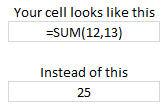
Formula not working – showing as text?
If you don’t see any error, but instead of seeing the result, all you see is your formula (like below), then check out Formulas not working page for information how to fix the problem.
Further Reading on Excel Formula Debugging
Formula Debugging using F9 Key
Learn to work with Circular References
Understand the difference between absolute and relative references
How to work with tables & structural references
Detect errors in your formulas [Office.com]
How to use new ERROR.TYPE formula to work with errors
Tell me how you debug formulas? What is the most common error you get?
What is the strangest and most confusing error you have seen? Please share in the comments so we can all have a laugh and find a way to fix the problem.


4 Responses to “Office 2010 Contest Winners are here!!!”
I while ago I wrote a post on selecting a couple of names from a range via an UDF
I could have been handy.... especially because I didn't win.... lol
http://xlns.lamkamp.nl/?p=14
Sweet! I won! Thank you so much, Chandoo! I'm really speechless! I'll look out for an e-mail from you. Again, I really appreciate it, and I can't wait to fire it up!
Sincerely,
Tom "this one" 🙂
Thank You... Thank You... Thank You... 🙂
Hi,
Don't want to ruin your party.. 😉 but I noticed that when you sort the list A2:B11 (step 2), the RAND function re-calculates the numbers so that they are different and in mixed order again. I had to paste the whole area as values first and then sort to get it to work.
Wonder if the same happened to you because in your list at least Greg has a higher value than Tom 🙂