
Lets say you are responsible for sales of 100s of products (which belong to handful of categories). You are looking at sales of each product in last month & this month. And you want to understand whether sales are improving or declining by category. How would you do it?
Turns out, this is not a difficult problem. In fact, this question is asked every day & answered using Advances vs. Declines chart.
You may have seen this chart in financial newspapers or websites. Shown below, Advances vs. Declines chart tells us how many items have advanced & how many have declined.
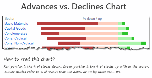
When should you use Advances vs. Declines chart?
As you can see, advances vs. declines chart does not give low level details about actual movement of values. Instead, it gives you a sense of what is going on. Use it in below situations:
- To get a feel of how values have changed over time.
- When you are dealing with data that constantly changes (sales, number of customers, defects etc.)
Create Advances vs. Declines chart in Excel
You can easily create this chart in Excel from raw data. Just follow below tutorial.
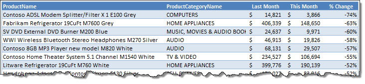
Step 1: Get the data & arrange it
You need at least 4 columns of data – item, category, previous value, current value
Once we have these, calculate % change in 5th column. Arrange data like below:
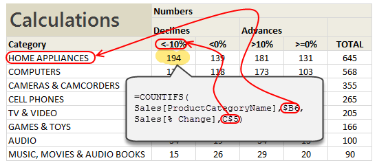
Step 2: Calculate Category-wise summaries
First list all unique categories in a column. Then using COUNTIFS formula, calculate the number of products declining & advancing.
The formula to count number of products going down by more than 10% is,
=COUNTIFS(Sales[category], Category name, Sales[% change], “<10%”)
[Related: Introduction to Excel SUMIFS / COUNTIFS Formulas]
Step 3: Calculate % break-ups for the chart
Once all the numbers are calculated, you can easily calculate the % split.
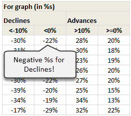
NOTE: Make sure you negate the % values for declines. This will ensure that our chart shows stacked bars on both sides of axis.
Step 4: Create a stacked bar chart from this data
Once all the numbers are in place, just select them and create a stacked bar chart. Your output should look like below:
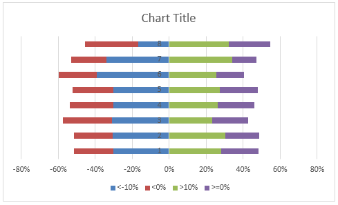
Step 5: Adjust chart series order if needed
You may notice that, our stacked chart bars are not in correct order. Excel would have plotted <10% and >10% series before <0% and >0% series. To fix this:
- Right click on the chart
- Go to Select Data
- Now, select the series area
- Using up / down buttons adjust the order of series
- Done!
See this demo to understand:

Step 6: Adjust the colors & format the chart
Unleash your creativity and format the chart as you see fit. Make sure you add legend (otherwise the chart becomes very difficult to read).
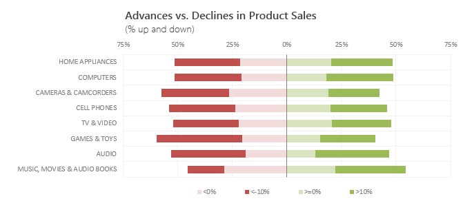
And you are done!
Download Advances vs. Declines chart template
Click here to download the chart template. Examine the formulas & chart settings to understand this better.
Do you use Advances vs. Declines chart?
I use variations of this chart often in my dashboards & reports. These charts are very concise and present a lot of information about distribution of changes.
What about you? Do you use advances vs. declines charts? How do you create them? Share your experiences & techniques using comments.
Looking to advance your charting knowledge?
If you want to one up your Excel awesomeness quotient & create kick-ass charts, then you are at the right place. Check out below tutorials & see how deep the rabbit hole goes:
- Visualizing tax changes over time using Excel
- Index Charts – to understand change over time
- Use Box plots to understand distribution of values
- Visualize monthly changes using Pivot Tables + Conditional formatting
Recommended: If all these sound exciting, you will incredibly benefit from our Excel School program, where we teach advanced charting & data analysis skills. Click here to know more & join us.


18 Responses
This is a great learning tip for category professionals or sales people! Thank you!
How did you get the category axis labels all the way to the left?
I can’t seem to move them
Thank you
@John.. Welcome to Chandoo.org and thanks for your comments.
To show labels at end, Right click on vertical axis, and set axis-labels position to LOW. This will move the labels to all the way left.
Hello Chandoo,
My question is: how could I add lables to the chart? I got the same chart as in Step 5 and I noticed there were no lables in it. How can I make my chart as beautiful as yours in Step 6. Thanks!
This is great.
Would there be a way of varying this so that instead of the centre being 0, it could be an average amount and the sides showing the over or under amount or % they are from the average score? Thanks.
buen grafico !
Dear Sir,
I want in excel sheet say various loan repaynebt or various fd mature date should be highlight as their time come near month/week.
could it possible.
Regards
Hemant
will join in later classes
Dear Chandoo,
thank you very much for this nice example. I can adjust it very well for your categories.
Happy Charting and greetings, SomeintPhia
Chandoo: I Think that we have an error in this example, May be in the symbols.
if you account cell by cell. you will realize that we don´t have the really result
MExico
I really felt pleasure after reading this.
Wow you just made excel charting so simple.
Thanks.
TellTheFolk
Hi Chandoo,
I tried the same on my sheets and it didn’t happen, I’ve been racking my brains to figure out what went wrong. I identified the range names, but all the values were coming out to be 0, I also don’t know how you defined “Sales”, I named the entire data array as that and even then none of the values were coming!
Hi Chandoo,
Thanks for this useful charting method. Please explain the way how the naming of the ranges is done in this sheet.
Thanks.
Hi Chandoo,
Thanks for this useful charting method. Please explain the way how the naming of the ranges is done in this sheet.
Thanks.
Hi Chandoo,
Thanks for this useful charting method. Please explain the way how the naming of the ranges is done in this sheet.
Thanks.
What do we take away and interpret from this chart?