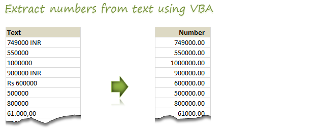
Last week we discussed how to extract numbers from text in Excel using formulas. In comments, quite a few people suggested that using VBA (Macros) to extract numbers would be simpler.
So today, lets learn how to write a VBA Function to extract numbers from any text.

Using VBA Function to Extract Numbers from Text in Excel
When using VBA to scan a text for number, the basic approach is like this:
- Read each character in a given text
- See if it is number
- If so, extract it
- Continue with next character
- Convert the extracted characters to a number
- Return that number
While this works fine, it also has some limitations.
For example, with above approach, A text value like “US $313,00.00” will be extracted as 3,130,000 not as 31,300.00
Depending on your data, you may have many such peculiarities. For example, here are 4 situations I ran in to:

Handling decimal points & thousand separators during extraction
When it comes to decimal points & thousand separators there are 2 conventions:
- 61,000.30 (Regular)
- 61.000,30 (European)
We do not need special treatment for regular format (61,000.30) as Excel & VBA are capable of dealing with these numbers by default.
To check if a text has European format number, we have to see if . occurs before ,
(Note: this method is not fool-proof, but should work well for most situations)
This can be done by using LIKE statement,
if text like "*.*,*" then

european = true

else

european = false

end if
Writing our getNumber() VBA Function
Once we put all these ideas together, we will have our getNumber() function. Watch below video to understand how to extract numbers from text using Excel VBA.
[Watch this video on our Youtube channel]
Download Number Extraction VBA Function
Click here to download the Extract Numbers using VBA workbook.
View code module to understand how getNumber function works.
Do you use VBA to extract numbers?
I often use VBA to clean raw data. Earlier I mentioned about cleaning phone numbers & spelling mistakes. I think simple functions like getNumber() can save us tons of time & let us focus on the important task – analyzing data.
What about you? Do you use VBA to clean data? What techniques & ideas you rely on? Please share your thoughts using comments.
New to Excel VBA? Take our crash course
Are you new to Excel VBA? If so, go thru below links to take our FREE VBA Crash course.
- What is VBA & Writing your First VBA Macro in Excel
- Understanding Variables, Conditions & Loops in VBA
- Using Cells, Ranges & Other Objects in your Macros
- Putting it all together – Your First VBA Application using Excel
- My Top 10 Tips for Mastering VBA & Excel Macros
If you want more,
I know you are thirsty for more. Why not join our Online VBA Classes and learn Excel VBA in step-by-step manner. Click here to know more.


8 Responses to “Create a Combination Chart, Add Secondary Axis in Excel [15 Second Tutorial]”
[...] Select the “daily completed” column and add it to the burn down chart. Once added, change the chart type for this series to bar chart (read how you can combine 2 different chart types in one) [...]
[...] set the height series to be plotted on secondary axis. Learn more about combining 2 chart types and adding secondary axis in [...]
[...] Excel Combination Charts – What are they? [...]
[...] To show the years, I have used another dummy series and plotted it on secondary axis (related: how to add secondary axis?) [...]
Thanks for this one!
[...] Choisissez la colonne « Daily Completed » et ajoutez-la au graphique. Une fois ajoutée, changez le type de graphique pour cette série à histogramme (lisez comment combiner 2 types de graphiques en un : combine 2 different chart types in one) [...]
How do i create a chart that has negative numbers on axis x and y and plot them correctly? I cannot seem to understand how to do this, please help.
Thanks.
Nat
You can also plot 2 or more Y axes in Excel using EZplot or Multy_Y from Office Expander.com
There is a demo version to try.
Cheers.