
This post builds on earlier discussion, How many hours did Johnny work? I recommend you to read that post too.
Lets say you have 2 dates (with time) in cells A1 and A2 indicating starting and ending timestamps of an activity. And you want to calculate how many workings hours the task took. Further, lets assume,
- Start date is in A1 and End date is in A2
- Work day starts at 9 AM and ends at 6PM
- and weekends are holidays
Now, if you were to calculate total number of working hours between 2 given dates, the first step would be to understand the problem thru, lets say a diagram like this:
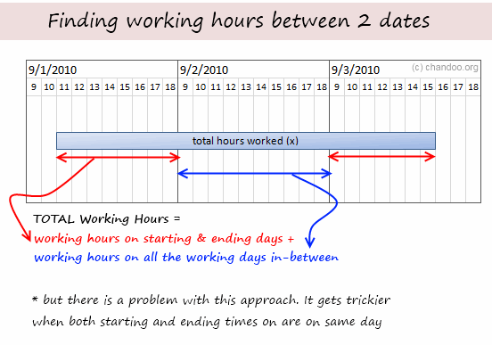
We would write a formula like this:
=(18/24-MOD(A1,1)+MOD(A2,1)-9/24)*24 + (NETWORKDAYS(A1,A2)-2)*9
See the above illustration to understand this formula.
Now, while this formula is not terribly long or ineffective, it does feel complicated.
May be we can solve the problem in a different way?!?
Michael left an interesting answer to my initial question, how many hours did Johnny work?
Pedro took the formula further with his comment.
The approach behind their formulas is simple and truly out of box.
Instead of calculating how many hours are worked, we try to calculate how many hours are not worked and then subtract this from the total working hours. Simple!
See this illustration:

So the formula becomes:
Total working hours between 2 dates – (hours not worked on starting day + hours not worked on ending day)
=NETWORKDAYS(A1,A2)*9 - (MOD(A1,1)-9/24 + 18/24 -MOD(A2,1))*24
After simplification, the formula becomes,
=NETWORKDAYS(A1,A2)*9 - (MOD(A1,1) -MOD(A2,1))*24 -9
=(NETWORKDAYS(A1,A2)-1)*9 +(MOD(A2,1)-MOD(A1,1))*24
Sixseven also posted an equally elegant formula that uses TIME function instead of MOD()
=(NETWORKDAYS(B3,C3)*9) - ((TIME(HOUR(B3),MINUTE(B3),SECOND(B3))-TIME(9,0,0))*24) - ((TIME(18,0,0)-TIME(HOUR(C3),MINUTE(C3),SECOND(C3)))*24)
Download the solution Workbook and play with it
Click here to download the solution workbook and use it to understand the formulas better.
Thanks to Pedro & Michael & Sixseven & All of you
If someone asks me what is the most valuable part of this site, I would proudly say, “the comments”. Every day, we get tens of insightful comments from around the world teaching us various important techniques, tricks and ideas.
Case in point: the comments by Michael, Pedro and Sixseven on the “how many hours…” post taught me how to think out of box to solve a tricky problem like this with an elegant, simple formula. Thank you very much Michael, Pedro, Sixseven and each and every one of you who comment. 🙂
Have a great weekend everyone.
PS: This weekend is my mom’s birthday, plus it is a minor festival in India. So I am going to eat sumptuously, party vigorously and relax carelessly. Next week is going to be big with launch of excel school 3.
PPS: While at it, you may want to sign up for excel school already. The free lesson offer will vanish on Wednesday.


49 Responses
At the risk of sounding like a jerk, the recommended approach, and Michael’s formula is basically the same as the one I proposed, with the exception that I used TIME(HOUR(),MINUTE(),SECOND()) instead of MOD.
I certainly agree that MOD makes for a shorter, and arguably simpler formula.
@Sixseven.. You are right. I missed your equally elegant formula in the heap of responses. Sorry. I have updated the post to include your name and formula. Thanks for pointing it out. 🙂
Hi Chandoo,
Maybe I’m missing something, but it looks like those formulas are not working correctly.
When Start Date= Friday 20, Aug 5:30PM and End Date= Monday 23, Aug 5:30PM
You get 9 hours
However, when Start Date= Monday 23, Aug 12:00AM and End Date= Monday 23, Aug 5:30PM
You get 17.50 hours
Can you clarify what are the correct results for both date ranges?
Thanks
@Elias… Sorry, but one of the assumptions of original problem was,
Starting time is an actual working hour. In your case 12:00 AM is not the case.
Try something like Start Date= Monday 23, Aug 10:00AM and End Date= Monday 23, Aug 5:30PM
You get correct answer.
Btw, the problem of fetching working hours between any given 2 dates without the condition that both start and end are not inside working hours could be even more interesting. Lets see if someone comes up with a clever answer for it.
Ok, I understand. Then, why the seven line of your file gets zero hours instead of four?
Star= Sunday 22, Aug 1:00PM and End= Monday 23, Aug 1:00PM.
Regards
@Chandoo..
Thanks. I appreciate the mention and the kind words. Also, I’m not sure if I would use the word “elegant” for my formula, but it get’s the job done… 🙂 This was a good exercise for me; I haven’t ever needed to use MOD before, so it was nice to see how others use it in action.
I like the homework assignments. Please keep them coming… 🙂
Chandoo:
.
Nice exercise.
.
My 2 cents would be:
=NETWORKDAYS(B3,C3,B3)*9-(B3-C3-INT(B3)+INT(C3))*24
.
This eliminated the MODs and the subtraction of one day from the initial Networkdays calc. Nothing wrong with MOD but in this case it is just being used to return the decimal part of each date, which can also be done by subtracting the integer portion as shown. This may be clearer for some readers.
The elimination of the subtraction is done by including the starting date in the list of holidays for the Networkdays function. We could also have chosen the ending date with the same result.
My new course, the Excel Hero Academy, includes a significant portion on creative formula crafting:
http://www.excelhero.com/blog/2010/09/excel-hero-academy—interested.html
.
Regards,
Daniel Ferry
excelhero.com
The original idea comes from http://www.cpearson.com/excel/DateTimeWS.htm. I just adapt it to this post.
A1=Start regular working hour
B1=End regular working hour
A3=Project Start Date & Hour
B3=Project End Date & Hour
=ABS(IF(INT(A3)=INT(B3),ROUND(24*(B3-A3),2),24*($B$1-$A$1)*(NETWORKDAYS(A3+1,B3-1)+INT(24*(MOD(B3,1)-MOD(A3,1)+($B$1-$A$1))/(24*($B$1-$A$1))))+MOD(ROUND(24*MOD(B3,1)-24*$A$1+24*$B$1-24*MOD(A3,1),2),ROUND(24*($B$1-$A$1),2))))
Regards
You can reduce the above formula using some auxiliary cells.
A1=Start regular working hour
B1=End regular working hour
C1=Total day working hours
A3=Project Start Date & Hour
B3=Project End Date & Hour
D3=Project Start Hour
E3=Project End Hour
=ABS(IF(INT(A3)=INT(B3),ROUND(24*(B3-A3),2),24*$C$1*(NETWORKDAYS(A3+1,B3-1)+INT(24*(E3-D3+$C$1)/(24*$C$1)))+MOD(ROUND(24*E3-24*$A$1+24*$B$1-24*D3,2),ROUND(24*$C$1,2))))
Regards
@Elias, could you check the original “biggest” Pearson formula?
You forgot this important MAX function to work correctly:
MAX(NETWORKDAYS(StartDT+1,EndDt-1,HolidayList),0)
@Daniel, with your last formula, it’s necessary to put start or end date into the HolidayList
@Chandoo, I agree with you when you says that the most valuable part of this site are comments and I would like that you write some comment on my blog.
The
=(NETWORKDAYS(A1,A2,Holidays)-1)*Hours +(MOD(A2,1)-MOD(A1,1))*24
Where:
– Holidays is an optional range of one or more dates to exclude from the working calendar.
– Hours are maximum working hours in a day.
Lets say Johnny doesn’t take any lunch breaks (he has developed a taste for those higgs bosons sandwich with positron milk shake).
@Pedro Wave –
.
That was the point.
@ Pedro-
.
Thanks for point that out, you are right we should include error control in all the proposed formulas.
.
I know that Person’s formula is huge, but I think we need something to control Start and End day working hours, not just total allowed work hours per day.
.
Also, it looks like all the formulas need to be fixed to return the correct result when the Start Date and End Date are on the same day but they are more hours than are allowed.
.
ie. Start Date = Thursday 19, Aug 9:00 AM and End Date = Thursday 19, Aug 9:00 PM.
.
.
Regards
@Daniel making your formula more general if you will permit me:
=NETWORKDAYS(B3,C3,Holidays)*Hours-(B3-C3-INT(B3)+INT(C3))*24
Where:
– Holidays is an optional range of one or more dates (including B3 or C3, ONLY ONE!) to exclude from the working calendar.
– Hours are maximum working hours without breaks in a day.
.
@Elias, Chandoo’s homework assumes a range of working hours without breaks.
.
If you want to expand the hours worked, you must indicate in the formula, by example: from 9:00 AM (min. start time) to 9:00 PM (max. stop time) are 12 hours and this formula works:
=(NETWORKDAYS(A1,A2,Holidays)-1)*12 +(MOD(A2,1)-MOD(A1,1))*24
.
If Johnny is working at midnight, should be an end date at 12:00 AM and a start date in the next line at same hour of next day.
.
For working breaks in the same or between two days, forces to think in another formula ways.
[Quote] Pedro.
“@Elias, Chandoo’s homework assumes a range of working hours without breaks”
[End Quote]
.
Pedro did you read Chandoo’s last paragraph on the fourth comment?
.
[Quote] Chandoo.
“Btw, the problem of fetching working hours between any given 2 dates without the condition that both start and end are not inside working hours could be even more interesting. Let’s see if someone comes up with a clever answer for it.”
[End Quote]
.
That’s why I came with Person’s formula.
.
Regards
@Chandoo, here it is my solution to the problem of fetching working hours between any given 2 dates without the condition that both start and end are not inside working hours:
=(DecimalHours*(NETWORKDAYS(B3,C3,HolidayList)-1)
+MAX(IF(NETWORKDAYS(C3,C3)0,MIN(MOD(C3,1),$D$26),$D$26),$D$25)
-MIN(IF(NETWORKDAYS(B3,B3)0,MAX(MOD(B3,1),$D$25),$D$25),$D$26))*24
.
It is included as Pedro Wave V.2 (Column K) in this file with other proposals until now:
http://cid-6b219f16da7128e3.office.live.com/view.aspx/.Public/working-hours-between-2-dates-data-solution2.xls
.
I also added in column L, worked hours by my civil servants or Spanish government employees.
Ok, here is one more huge option.
A1=DayStart time, B1=DayEnd Time
A3=SartDate, B3=EndDate
=IF(INT(A3)=INT(B3),MIN(B3-A3,$B$1-$A$1)*NETWORKDAYS(A3,A3,HolidayList),($B$1-MIN(MAX(MOD(A3,1),$A$1),$B$1))*NETWORKDAYS(A3,A3,HolidayList)+(MAX(MIN(MOD(B3,1),$B$1),$A$1)-$A$1)*NETWORKDAYS(B3,B3,HolidayList)+MAX(NETWORKDAYS(A3+1,B3-1,HolidayList),0)*($B$1-$A$1))*24
Regards
@Chandoo, my last formula is incomplete due to lack of signs minor and major in my last comment, so it is better seen at the K column of my last file. Only worked hours are added between regular start and end working hours, excluding hours into holiday dates.
@Elias, I modified your formula in my last file including references to a new HolidayList sheet and to DecimalHours as:
= $D$26 – $D$25
where:
$D$25 = Start regular working hour
$D$26 = End regular working hour
@Daniel, in the G (Start Date) and H (End Date) columns are your formulas without including HolidayList. Could you give us a solution for the argument to exclude other Holidays dates?
@ Pedro. I like your last formula, I think it would be better if it includes the HolidayList in all NETWORKDAYS function. Just in case the StartDate or EndDate are holidays.
@ Chandoo. My earliest post (around 9:00AM CT) didn’t get post, any idea why this might happen?
Regards
@Elias, thanks for reminding me. I just added the reference to HolidayList in all formulas, except into Daniel Ferry formulas, in this new file:
http://cid-6b219f16da7128e3.office.live.com/view.aspx/.Public/working-hours-between-2-dates-data-solution3.xls
I’ve included your last formula in column M. I have marked in orange half-hour discrepancy in row 19. You can keep an eye on it?
You will agree with me that the Chip Pearson formula adds nothing to our latest proposals for resolving the problem posted by Chandoo.
.
@Chandoo, when a work day starts at 9 AM and ends at 6PM there are only 9 worked hours and you represent 10 hours in your images, which I corrected in my uploaded files.
I think this one works better than my previous one.
.
A1=DayStart time, B1=DayEnd time and C1=B1–A1
A3=SartDate and B3=EndDate
.
=(
($A$1-MIN(MAX(MOD(A3,1),$A$1),$B$1))*
NETWORKDAYS(A3,A3,HolidayList)+
(MAX(MIN(MOD(B3,1),$B$1),$A$1)-$B$1)*
NETWORKDAYS(B3,B3,HolidayList)+
MAX(NETWORKDAYS(A3,B3,HolidayList),0)*$C$1
)*24
.
Regards
@Elias, your formula give me for:
Monday 16, Aug 10:00 AM to Tuesday 17, Aug 1:00 PM = 11 h (before 12 h)
Sunday 22, Aug 1:00 PM to Monday 23, Aug 1:00 PM = 0 h (before 4 h), etc…
Your above formula was better! Only one different date, now 7…
Could you try again?
@Pedro. I get the correct results, maybe is the way I pasted the formula. Let’s try this one that uses the same cells you are using in your file.
=(($D$28-MIN(MAX(MOD(B3,1),$D$28),$D$29))*NETWORKDAYS(B3,B3,HolidayList)+(MAX(MIN(MOD(C3,1),$D$29),$D$28)-$D$29)*NETWORKDAYS(C3,C3,HolidayList)+MAX(NETWORKDAYS(B3,C3,HolidayList),0)*DecimalHours)*24
Regards
Hi guys, sorry but what is “Decimalhours” in this post
@Elias, error was not yours, but mine since I transformed it wrong to try.
I entered your formula as Elias V.3 in column N in the next file:
http://cid-6b219f16da7128e3.office.live.com/view.aspx/.Public/working-hours-between-2-dates-data-solution4.xls
.
@ Chandoo, my previous formula expressed in two more ways:
=(DecimalHours*(NETWORKDAYS(B3,C3,HolidayList)-1)+ MAX(IF(NETWORKDAYS(C3,C3,HolidayList)=0,$D$29,MIN(MOD(C3,1),$D$29)),$D$28)-MIN(IF(NETWORKDAYS(B3,B3,HolidayList)=0,$D$28,MAX(MOD(B3,1),$D$28)),$D$29))*24
.
=(DecimalHours*(NETWORKDAYS(B3,C3,HolidayList)-1)+ IF(NETWORKDAYS(C3,C3,HolidayList)=0,MAX($D$28,$D$29),MAX($D$28,MIN(MOD(C3,1),$D$29)))-IF(NETWORKDAYS(B3,B3,HolidayList)=0,MIN($D$28,$D$29),MIN($D$29,MAX(MOD(B3,1),$D$28))))*24
I entered this last formula as Peter V.3 in column O on the attached file.
I just saw that my last formula can be simplified since start is less than end of regular working hours:
=(DecimalHours*(NETWORKDAYS(B3,C3,HolidayList)-1)+ IF(NETWORKDAYS(C3,C3,HolidayList)=0,$D$29,MAX($D$28,MIN(MOD(C3,1),$D$29)))- IF(NETWORKDAYS(B3,B3,HolidayList)=0,$D$28,MIN($D$29,MAX(MOD(B3,1),$D$28))))*24
Or are exactly equal for some workers!
hi chandoo,
I am not able to understand why 9 is used in that formula…! can u please explain…
can this formula be adapted to account for the working hours chaging based onthe day of the week.
My problem is that my working hours are
Monday to Friday 08:00:00 to 17:30:00
Saturday 09:00:00 to 16:00:00
Sunday 09:00:00 to 14:00:00
i am really struggling to find an answer for this??
Cheers
Donna
@Donna, It may be a little late but here’s my solution to your problem when working hours are changing based on the day of the week.
In Excel 2010, sum this formula 3 times, once for each range:
=IF(A10>B10,0,+$D$2*(NETWORKDAYS.INTL(A10,B10,Range1,Holidays)-1)
+IF(NETWORKDAYS.INTL(B10,B10,Range1,Holidays)=0,MAX($B$2,$C$2),MAX($B$2,MIN(MOD(B10,1),$C$2)))
-IF(NETWORKDAYS.INTL(A10,A10,Range1,Holidays)=0,MIN($B$2,$C$2),MIN($C$2,MAX(MOD(A10,1),$B$2))))
Where:
Range1 = “0000011” (Monday to Friday)
Range2 = “1111101” (Saturday)
Range3 = “1111110” (Sunday)
Better download an Excel template from my blog:
http://pedrowave.blogspot.com.es/2013/03/hours-between-dates.html
Excel 2003 and 2007: Column D, using the auxiliary columns E:K
Excel 2010 and later: Column C, using the new WORKDAY.INTL function
How to Calculate working hours when holidays are not off but have different working hours?
I am calculating difference of hours betweens two days excluding weekends but i am getting 9hr less in my result. In my project they are calculating on severity basis so i include IF command in the below formula.
I am using the below formula:
=IF(B30<3,E30,((NETWORKDAYS(C30,D30)-1-MOD(C30,1)+MOD(D30,1))*24))
I am using the above formula for below example but i am not getting the rigt answer.
B30 (Severity =3 ) C30 (Opentime = 4/10/2013 3:04) D30 (Closed time = 4/14/2013 15:41) E30 (Total time including weekends = 108.6141)
correct ans 68.96 hrs
Here C30 is start time and D30 is closed time
I am getting 60.61 hrs but the correct answer is 68.96 hrs.
Ticket is opened on 10th April at 3:04am and closed on 14th April at 15:41. Here Business days are 10,11 and 12 April and if we calcluate it manually then its comes as below:
(As open time is 3:04 AM so we have 20:96 hrs in hand from 24 hrs)
20:96 hrs for 10th Apr + 24 hrs for 11th Apr + 24 hrs for 12th Apr = 68.96 hrs but i am getting only 60.61 hrs by the above formula.
Please help me in this.
@Prashant
E30 should be:
=(D30-C30-((INT(D30)-INT(C30))-NETWORKDAYS.INTL(C30,D30-1,17)))*24
= 84.6166667
Made up of:Date Hours
10 0.87
11 1.00
12 1.00
13 -
14 0.65
Days 3.53
Hrs 84.61666667
Thanks for the quick response.
But we are not considering weekends i.e. Saturday and Sunday.
Can you please help. Thanks in advance.
Here 13 and 14 April is Weekends can you please exclude them from this formula.
Thanks..
Could I throw this one open, as it is relevant in the project I’m currently undertaking.
What if the End Date is before the Start Date?
Based on a normal working day m-f (08:00-17:00) and using the dates and times as:
Start: Wed 14/8/13 8am
End: Tues 13/8/13 4pm
My reason for this. If something arrives in the office (say telephone callback) at 4pm on Tues, we have a maximum 3-hour turnround to action it, so the action date would be the following day. The answer I’m looking to achieve for the above example is -1.00 hrs, but all I get is -19.00 hrs: 4-5pm = 1 hour and then start of next day would be 8am. The answer I’m getting is including out-of-office hours which is not what I’m after.
Sounds strange, but hope I’ve explained it enough. I still wish to be able to have a start date earlier than the end date.
Regards
Paul S
Request Created Time Request Closed Time ? No of hours
13.09.2013 07:12 PM 18.09.2013 11:11 AM need a formula to calculate no of hours considering 16 hrs of working time
Hi Chandoo
Thanks for the blog which is great help for my project.
I have managed to custom the formula and it works fine but it throws error for below start and end date (all GMT).
Start: 21/06/2015 17:49
End: 22/06/2015 06:55
=TEXT((24*(NETWORKDAYS(A4,B4,RDATA!$AC$2:$AC$71)-1)-24*((MAX(MOD(A4,1),MOD(B4,1))-MIN(MOD(A4,1),MOD(B4,1)))))/24,”dd/hh/mm”)
Not sure what the error is but will be helpful if you can point out anything in the formula.
Best
Ram
Not sure this may help other but managed to get the desired result with this..
=IF(AND(DAY(A2)DAY(B2),MONTH(A2)MONTH(B2),OR(MOD(A2,1)>MOD(B2,1),MOD(A2,1)<MOD(B2,1))),TEXT((24*(NETWORKDAYS(A2,B2,RDATA!$AC$2:$AC$71))-24*((MOD(A2,1)-MOD(B2,1))))/24-1,"d/hh/mm"),IF(AND(DAY(A2)DAY(B2),MONTH(A2)=MONTH(B2),MOD(A2,1)<MOD(B2,1)),TEXT((24*(NETWORKDAYS(A2,B2,RDATA!$AC$2:$AC$71))-24*((MOD(A2,1)-MOD(B2,1))))/24-1,"d/hh/mm"),IF(AND(DAY(A2)DAY(B2),MONTH(A2)=MONTH(B2),MOD(A2,1)>=MOD(B2,1),MAX(A2:B2)-MIN(A2:B2)>=6),NETWORKDAYS(A2,B2,RDATA!$AC$2:$AC$71)-IF(MOD(A2,1)<=MOD(B2,1),0,1)-1&"/"&TEXT(B2-A2,"hh")&"/"&RIGHT(TEXT(B2-A2,"hh:mm"),2),IF(AND(DAY(A2)DAY(B2),MONTH(A2)=MONTH(B2),MOD(A2,1)>MOD(B2,1),MAX(A2:B2)-MIN(A2:B2)<6),NETWORKDAYS(A2,B2,RDATA!$AC$2:$AC$71)-IF(MOD(A2,1)<=MOD(B2,1),0,1)&"/"&TEXT(B2-A2,"hh")&"/"&RIGHT(TEXT(B2-A2,"hh:mm"),2),IF(AND(DAY(A2)=DAY(B2),MONTH(A2)=MONTH(B2),MOD(A2,1)<MOD(B2,1)),NETWORKDAYS(A2,B2,RDATA!$AC$2:$AC$71)-IF(MOD(A2,1)<=MOD(B2,1),0,1)-1&"/"&TEXT(B2-A2,"hh")&"/"&RIGHT(TEXT(B2-A2,"hh:mm"),2),"")))))
Can someone please assist with the following …
Workday starts at 08h00
Lunch 12h00 to 13h00
Workday ends at 17h00
I need to calculate the # of hrs worked … excluding lunch, excluding weekends and holidays.
A1=workdayStart
B1=lunchStart
C1=lunchEnd
D1=workdayEnd
A4=FromDateAndTime
B4=EndDateAndTime
C4=Total # of hrs worked … excluding lunch, excluding weekends and holidays
I have tried various options, but seems to be missing something here.
thanks
talana
hi Talana,
wondering if you already have the answer yet, could you share with me? I got the same problem also need the formula working in excel 2007..
thx
Hi Talana and Anton,
Regarding the request includes break time, I have just considered that within a day, there are two periods with different start time and end time:
A1=workdayStart
B1=lunchStart
C1=lunchEnd
D1=workdayEnd
A4=FromDateAndTime
B4=EndDateAndTime
1st period:
A1=workdayStart
B1=lunchStart
2nd period:
C1=lunchEnd
D1=workdayEnd
Holidays can be taken into account, ex.$E$2:$E$5
Only the time within these two periods considered working time.
I have found this formula works well for me:
(NETWORKDAYS(A4,B4,$E$2:$E$5)-1)*(($D$1-$A$1)-($C$1-$B$1)+IF(NETWORKDAYS(B4,B4),MEDIAN(MOD(B4,1),$B$1,$A$1)-MEDIAN(NETWORKDAYS(A4,A4,$E$2:$E$5)*MOD(A4,1),$B$1,$A$1))+IF(NETWORKDAYS(B4,B4),MEDIAN(MOD(B4,1),$D$1,$C$1)-MEDIAN(NETWORKDAYS(A4,A4,$E$2:$E$5)*MOD(A4,1),$D$1,$C$1))
(NETWORKDAYS(A4,B4,$E$2:$E$5)-1)*(($D$1-$A$1)-($C$1-$B$1)+IF(NETWORKDAYS(B4,B4),MEDIAN(MOD(B4,1),$B$1,$A$1)-MEDIAN(NETWORKDAYS(A4,A4)*MOD(A4,1),$B$1,$A$1))+IF(NETWORKDAYS(B4,B4),MEDIAN(MOD(B4,1),$D$1,$C$1)-MEDIAN(NETWORKDAYS(A4,A4)*MOD(A4,1),$D$1,$C$1))
=> i forgot to erase holiday in some part of old formula, holiday should appear once only
Hi,
I want to calculate the hours between two dates which exclude hours friday 6:00 P.M to Sunday 6:00 P.M
Hello,
I am not an expert in excel formulas, I have spent almost 3-4 hrs to understand this formula =(NETWORKDAYS(A1,A2)-1)*9 +(MOD(A2,1)-MOD(A1,1))*24
Dates are:
Monday 16, Aug 10:00 AM (B3)
Tuesday 17, Aug 1:00 PM (C3)
Things that I don’t understand:
=(NETWORKDAYS(A1,A2)-1)*9
why we subs 1, I thought if we dont subs then it will give 18 which seems logical i;e total working hours for two days
+(MOD(A2,1)-MOD(A1,1))*24
by multiplying 24, means we want to convert it to hours term, which gives us 3 (10 AM to 1 PM)
But then 18-3 gives us 15 which is incorrect.
I am lost. Please explain the formula if anyone can.
Hello,
Can someone explain the simplification process of the formula:
FROM
=NETWORKDAYS(A1,A2)*9 – (MOD(A1,1)-9/24 + 18/24 -MOD(A2,1))*24
TO
=NETWORKDAYS(A1,A2)*9 – (MOD(A1,1) -MOD(A2,1))*24 -9
=(NETWORKDAYS(A1,A2)-1)*9 +(MOD(A2,1)-MOD(A1,1))*24
Hi,
Just wondering if anyone has been able to modify the formula to deduction out time taken for lunch? Using this to determine time off taken so could have a start of 04/04/2017 11:00 AM and an end of 04/04/2017 4:30 PM. As lunch time is not included in the time off taken, in this example the total time off would be 5 hours (less 0.5 hrs for lunch).
is it possible to do this in DAX?
The attached discussion is my attempt to improve Chip Pearson’s formula. The suggested formulas don’t require that the beginning and ending times bracket the work shift.
The formulas use four named ranges:
beginning and ending (of the period being measured), which include both date and time elements
ShiftBegin and ShiftEnd which include only the times for the start and end of the work shift
The formulas are only valid when starting and ending dates are different!
By way of explanation:
1. Time consumed on the first and last days of the interval is figured using the MOD expressions.
2. Time consumed in the interior of the interval is figured using (NETWORKDAYS -2)*Shift length. Since NETWORKDAYS excludes weekends, you may include those weekend days by using (INT(ending) – INT(beginning) -1) instead of (NETWORKDAYS-2).
3. If the work shift spans midnight, its duration may be calculated directly using MOD. If not, the overall elapsed time (excluding intervening days) less MOD(rest end – rest start,1) is used instead.
MOD(ending,1) returns just the time portion of the date/time serial number
MOD(ShiftEnd – ShiftBegin,1) returns the number of hours in the shift, regardless whether that shift spans midnight or not. This expression assumes the number of hours in the interval is less than 24.
Work time
=IF(ShiftEnd>ShiftBegin,
(MOD(ending,1)+1-MOD(beginning,1)) –
MOD(MIN(MOD(ending,1),ShiftBegin)-MAX(MOD(beginning,1),ShiftEnd),1),
MOD(MIN(MOD(ending,1),ShiftEnd)-MAX(MOD(beginning,1),ShiftBegin),1))
+ MAX(0,NETWORKDAYS(beginning,ending)-2)*MOD(ShiftEnd-ShiftBegin,1)
Rest time
=IF(ShiftEnd>ShiftBegin,
MOD(MIN(MOD(ending,1),ShiftBegin)-MAX(MOD(beginning,1),ShiftEnd),1),
(MOD(ending,1)+1-MOD(beginning,1)) –
MOD(MIN(MOD(ending,1),ShiftEnd)-MAX(MOD(beginning,1),ShiftBegin),1))
+ MAX(0,NETWORKDAYS(beginning,ending)-2)*MOD(ShiftBegin-ShiftEnd,1)
Ahaa, C’est un dialogue délicat sur cette paragraphe dans
cette place sur cette webpage, j’ai lu tout ça, alors maintenant je commente aussi ici.