
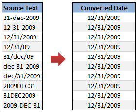
Sometimes when we import data from another source in to excel, the dates are not imported properly. This can be due to any number of reasons, including,
- The date format is different from one that is understood by excel
- The data has some extra spaces, other characters before and after the date values.
- The dates are formatted for another country (or date system) and hence your version of Excel wont recognize them.
- The separator between date, month and year is not a known separator (for eg. 12=DEC=2009 instead of 12-Dec-2009), etc.
In this post, we will learn some tricks and ideas you can use to quickly convert text to dates.
Technique 1: Use Text to Columns Utility
- First copy the source data and paste it in a text file (open Notepad and paste there).
- Now copy the values from text file and paste them in Excel.
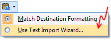
- At this point, Excel will prompt you for using “Text to columns” utility (or Text Import Wizard as it is called in Excel 2007)
- Go to the Text Import Wizard (or Text to Columns dialog).
- Leave defaults or make changes in step 1 & 2.
- In step 3, select “Date” and specify the format of the date – like YMD, MDY, DMY, YDM, MYD or DYM. It doesn’t matter what is the format of source date, month or year is. Excel can smartly understand them.
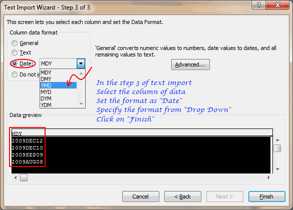
- Click “Finish”.
That is all. Your text dates are now converted to excel understandable dates.
Technique 2: Using Formulas to Convert Text to Dates
- Paste the data in a column (say “A”)
- Now depending on the format of source data, write one of the below formulas to convert text to dates.
Using DATEVALUE formula
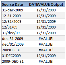
DATEVALUE formula tells excel to fetch the date from a given input. It is a smart formula capable of converting dates stored as text to excel understandable date format. To convert a text in cell A1 to date, you just write =DATEVALUE(A1)
However, DATEVALUE formula has some limitations. It cannot process all types of dates. For eg. I have shown a few sample dates along with corresponding DATEVALUE output.
Readjusting Date Text so that it works with DATEVALUE formula
Whenever possible, your next best option is to re-adjust the source data text so that it can be understood by DATEVALUE formula. Here is an example.
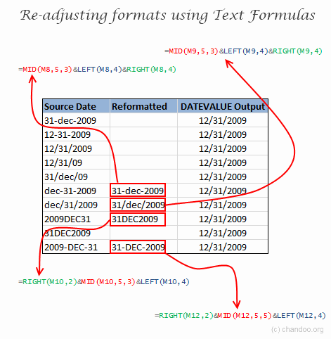
We can use the text formulas like LEFT, RIGHT and MID to extract portions of the date text and then regroup them using & operator to create meaningful date text format that would be understood by DATEVALUE formula.
Technique 3: Using DATE formula to Convert Text to Dates
If your data has separate columns for date, month and year, you can use DATE formula to convert the data to dates like this:
=DATE(year,month,day)
For eg. =DATE(2009,12,31) will give the date 31st December, 2009.
Bonus Technique: Converting Dates to Text
If you want to convert excel dates to text values (for your report or some other purpose), you can use the TEXT formula like this:
=TEXT(A1,"DD-MMM-YYYY") will convert date in Cell A1 to DD-MMM-YYYY format. You can pass any other date / time formats to TEXT formula as well. [more: tutorials on TEXT() formula]
How do you deal with troublesome dates?
Of course, if it is a real date, we can always bolt. But if it is a date in the data, we need some tools to deal with it. I used to rely on formula based methods to clean the dates. But recently I discovered the import-text date conversion method. This is very powerful and straightforward. Now, I use it whenever possible to clean up my date data.
What about you? How do you deal with buggy / faulty dates in Excel?
Recommended Articles:


62 Responses
Some good ideas. I had to do something like this recently, I can’t remember the exact format of the input data, but it was something like “01.01.2010” and using Edit, Find and Replace, to find “.” and replace with “/” was enough. I’m not suggesting this is better than any of the methods already listed.
you are Awsome,, Many Many thanks for your easy and straight forward solution 🙂
Concur! Awesome so elegant and simple 🙂
Great Post !!
the DATE function is great for all of us not using MMDDYY format, because we can manipulate the string containing the date to proper present it, when is not in the format we want to.
also, when importing text files, sometimes I’ve found the need to create an auxiliary list for the months, and also adding the 2 first digits to the year, before even pass the result as argument to the DATE function.
Rgds.
I created a macro with a hotkey for this. Our database stores dates in ‘4/1/2002 12:00:00 AM’ format which shows up in Excel as ’00:00.0′. Here is the macro:
Sub format_date()
‘
‘ format_date Macro
‘ format selection to date
‘
‘ Keyboard Shortcut: Ctrl+d
‘
Selection.NumberFormat = “m/d/yyyy”
End Sub
Hi Chandoo
Text to column dialog box can be triggered from “Text to Columns” button on Data Tab. With this you can easily avoid the steps to copy source data to note pad file. Just select the data cells on your excel file and start directly from step 4 in Technique 1 list above using Text to Column button on Data Tab.
Thanks
Yogesh Gupta
Hi Chandoo,
I am glad you published this post. I have been using the “text to column” tool for quite some time. It really comes in handy in cleaning up the data and even sometimes for creating the data for uploads (for example, for testing). This tool is very useful when you want to change the data that excel understands to the data what your software understands. In the process of changing the data a combination of text to column, concatenate formulae etc can be used and bingo!!! you get the data ready to uploaded in system (most of the time the coders leave this flabbergasted – “Man, how did you do that?? that was quite a DATA, boy”)……;)
Another example of the use of text to column is to trifurcate a name in three columns namely First Name, Middle Name and Last Name or Surname.
Cheers!!!!
Pankaj Verma
@Gerald.. good input on using find / replace. Thanks for sharing it. 🙂
@Martin: I guess excel asks you for the date system (19xx or 20xx) when you import dates with 2 digit year codes.
@Martin: Very good and very simple macro. Thanks for posting it for all of us.
@Yogesh: Thanks for pointing that out. In fact, I had the text-to-columns on my quick access bar because my office comp uses european date system and all the incoming CSVs used US date system.
@Pankaj: good use of text to columns to split names. I use it often to clean up urls, email ids and other stuff too.
For those who might be interested in a VB solution, below is a macro that will take a column of text strings that are meant to be dates and convert them into dates. The macro will convert the following patterned text into real dates as indicated (“y” is a year digit, “m” is a month digit or letter depending on if there are 1, 2 or 3 of them in the pattern, and “d” is a day digit)…
yy (January 1st assumed)
m/d or m/d/ (current year assumed)
m/dd or m/dd/ (current year assumed)
mm/d or mm/d/ (current year assumed)
mm/dd or mm/dd (current year assumed)
mm/dd/yy
mm/dd/yyyy
mmdd (current year assumed)
mmddyy
mmddyyyy
dmmmyyyy or ddmmmyyyy
yyyymmmdd or yyyymmmd
Note that the date order is month/day. I **think** the code will work if your system uses day/month ordering; but, since I have never done any international programming, I don’t know that for sure. I would appreciate feedback from those whose date order is day/month. Okay, anyway, here is the macro (set the two Const statement assignments to match your actual setup)…
Sub ConvertToProperDates()
Dim D As Date, S As String, Sin As String, X As Long, LastRow As Long
Const StartRow As Long = 2
Const DateCol As String = “A”
LastRow = Cells(Rows.Count, DateCol).End(xlUp).Row
On Error Resume Next
For X = StartRow To LastRow
Sin = Cells(X, DateCol).Value
S = Trim(Replace(Replace(Sin, “/”, “-“), Application. _
International(xlDateSeparator), “-“))
If Right(S, 1) = “-” Then S = Left(S, Len(S) – 1)
If Len(S) = 2 Then
D = DateSerial(S, 1, 1)
ElseIf InStr(S, “-“) Then
D = CDate(S)
ElseIf S Like “#[A-Za-z][A-Za-z][A-Za-z]####” Or _
S Like “##[A-Za-z][A-Za-z][A-Za-z]####” Then
D = CDate(Val(S) & “-” & Mid(S, Len(S) – 6, 3) & “-” & Right(S, 4))
ElseIf S Like “####[A-Za-z][A-Za-z][A-Za-z]#” Or _
S Like “####[A-Za-z][A-Za-z][A-Za-z]##” Then
D = CDate(Left(S, 4) & “-” & Mid(S, 5, 3) & “-” & Mid(S, 8))
Else
S = Format(S, “!&&-&&-&&&&”)
If Right(S, 1) = “-” Then S = Left(S, Len(S) – 1)
D = CDate(S)
End If
If Err.Number Then
Cells(X, DateCol).Value = “?? ” & Sin & ” ??”
Err.Clear
Else
Cells(X, DateCol).Value = D
End If
Next
End Sub
Thank you so much, Rick! With a bit of changes to the code, I was able to tailor-fix my problem with bad date formatting (i.e. Mar 4 2017 as text to 04-03-2017). 🙂
Just a follow up on my macro… I notice that code got posted with some character substitutions that you will need to correct in order to make the code work in your VB code window… after you copy/paste the above code into your VB code window in Excel, change the beginning quote marks (“) and ending quotemarks (”) to normal quote marks; and in the three statements containing the Len(S) function calls, change the elongated minus signs that were placed after them to normal minus signs. Everything else looks like is copy/pastes just fine.
Rick this is giving an error: ‘Type mismatch’ for LastRow = Cells(Rows.Count, DateCol).End(xlUp).Row
Text to column is very great menu to convert data type.
Hi
Thanks for the tips Chandoo.
Unfortunately I have an issue that does not appear to be addressed in various blogs that i have come across yet. I am pulling dates into Excel as text, looking like this: 010805, which ought to read as 01/08/2005 (dd/mm/yyyy). However, using technique 3 as described by Chandoo above, it converts to 10/08/2005 so it is ignoring the first “0” in my text.
I have also tried using a custom format date to dd/mm/yyyy, but unfortunately this option returns a date of the text as 31/07/1929.
Any suggestions to get around this issue?
Thanks
Robapottamus
first of all format the cells where your date gets imported to as text – formatcell-tex
import your date(without separator)
assuming your imported date is in A1
enter formula
=(LEFT(A1,2)&”/”&MID(A1,3,2)&”/”&RIGHT(A1,2))+0
0 is added to bring it to number format
@Robapottamus
Add a helper column
=DATE(2000+RIGHT(A2,2),MID(A2,3,2),LEFT(A2,2))
Copy down
Copy and paste as values
Format as Dates with dd/mm/yyyy
Desperate for help!
I work with importing data into excel often from different tables within our system. The problem is that different tables have different formats for storing a date field. What I have not seen addressed is what happens when date fields are stored as NUMERIC data types instead of text?
For example,
Table_1 (The easy table): Field name [Customer_Add_Date] formatted as CCYYMMDD stored as a numeric field type. So to convert this to a date, I have to use a date conversion =DATE(LEFT([Customer_Add_Date],4),MID([Customer_Add_Date],5,2),RIGHT([Customer_Add_Date],2))
Table_2 (The painful table): This table stores dates in a numeric field type as YYMMDD. So if there was a payment transaction on January 9, 2000, the data would look like this “109”. So I have to qualify using lengths and it is a painful experience.
Has anyone run across this before? Does anyone have a user-defined function that can convert numeric field types into dates??
Thanks!!!
I use CNTRL+H and replce all “- and /” with Blanks and then use Alt+D+T convert it to Date Format
Can you please tell me How to Convert dates to text.
Like some one enter 3/1/2012 , it should look 3 jan.
In Excel 2010.
Thanks
Ritesh
@Ritesh
Select the cell
Ctrl 1
On the Number Tab, select Custom
in the Type: Box enter
d mmm
Apply
Have a read of
http://chandoo.org/wp/2008/02/25/custom-cell-formatting-in-excel-few-tips-tricks/
Dear All,
Need your help plz..
I have imported some data from text to excel and got a text format in the cell as “LW117541 20/04/2011” and another cell with “LW118979 08/07/2011” then I wrote a formula to get the date separately as “=RIGHT(G10,10)” and separated the date and now i couldnt convert to any of the date format. though my cell value is “21/04/2011” i couldnt understand in what format it is? then based on some of the above comments I just replaced “/” with “-” and found to format again and only the second date as mentioned above has changed “08/07/2011” but the first date “20/04/2011” seems to have the old format.
Kindly help!!
Hi,
my machine gives date in the format 19.06.2012 and I simply use “substitute” formula to make it understand to excel and also calculate the differance in dates
Thanks
Jignesh Pandya
you just save me from tedious work of converting text day to excel date.
Thank you for your generosity.
Hi, I am receiving the automated excel reports generated from online tool. The date formats are shown in a following way:May 14 2012. I wanted to make a calculation of the future dates – e.g. review in 365 days from given date but it shows the VALUE# error. I’ve tried to check the date format using the text import wizard but it just doesn’t work – it doesn’t change a date format, it still shows me the error in the formula :/
@Emilia
Can you post a sample file, Refer: http://chandoo.org/forums/topic/posting-a-sample-workbook
Showing some of the date values
Hi I receive a file with dates in the following format and I spend a lot of time converting them into a useable format; can anyone suggest an easy to understand / implement solution, please….
June 15, 2012 9:59 AM
May 24, 2012 12:15 PM
April 12, 2012 10:26 AM
March 23, 2012 8:49 AM
I dont need / want the time element. I simply want e.g. 15/06/2012
Thanks.
Text to columns
delimeters – check space
finsh
format to ‘dd/mm/yyyy”
done
Just want to say THANK YOU! Really appreciate the pedagogical approach on this site. The chart showing the example of date formats and what they’ll retreive via the DateValue formula let me to a solution in no time. THANKS AGAIN!
Your Technique 1 saved me Hours and Hours of painstaking task. Thank you Chandoo.
All i can say is BRILLIANT!! Technique 1 worked well for me. Many Thanks and much appreciated
4/29/2013 6:44:00 AM
The above date and time is in general format .need to covert to date and time format(yyyy-mm-dd hh:MM:SS).Tried with text formaula but not giving any answer.
great work!! Saved lot of my time.
Thank you so much
Hi,
I get Dates in a software generated report as “Thu 4/18/2013 2:15 PM” in text format.
I use Date(mid(search(“/”,… to extract the date but it is problematic because / is placed differently in dates like 4/8/2013, 4/18/2013 and 11/18/2012.
Is there some simple way to extract dates from such a text format?
Thanks. I was able to use mid and right to reformat the dates!
I need to create a macro that changes the date on the current formula in about 30 Cells to the current date -1 (Previous day)
The formula looks like this
=+’Y:\2014\Shifts\July 2013\[18 July 2013.xls]Shifts’!$D$12
The 18 July 2013 needs to change when the macro runs to the current date – 1
Your help would be appreciated.
What about a date starting from a Century like 1131122 (22nd Nov 2013).
this is what I use at work, but I completely DO NOT understand why it works. Anybody would like to shed some light?
=DATE(MOD(INT(A1/10000),100)+2000,MOD(INT(A1/100),100),MOD(A1,100))
thanks in advance,
Penelopy
Superb information,thanks Chandoo
Hello,
I am trying to convert Tue Dec 10 12:37:13 PST 2013 to mm/dd/yy format and none of these techniques work. Am I doing something wrong?
Please help!
Thanks in advance,
Dimple.
The above technique worked fine for me also.
However, my problem now is how to find a MAX or MIN or AVERAGE a range of MAX & MIN ‘Time’ cells in HH:MM:SS format (other than just sorting them).
MAX = is the latest time
MIN = is the earliest time
AVERAGE a range of MAX or MIN values of HH:MM:SS time.
Awesome! I spent an hour trying to figure this out! great article.
Hi,
This was an issue that was giving trouble to me for a long long time. Thanks to this piece of Excel wisdom, that was solved.
Thanks again!
Nandan
I have date format in the following manner in the excel which is in string format
Apr 1, 2016 12:37:06 PM
Apr 2, 2016 12:00:00 AM
Apr 1, 2016 9:50:22 AM
Apr 1, 2016 12:09:38 PM
Apr 1, 2016 6:53:03 PM
Apr 1, 2016 1:02:10 PM
I have tried converting it from general to date however excel still does not recognize it as date format. Need your advise as what can I try more to solve this.
@Nik
Can you post the question at the Chandoo.org Forums http://forum.chandoo.org/
Attach a sample file because as soon as I copy and paste this text, Excel recognises it as valid Dates and Times
I am trying to convert date codes, they are not always standard. They can be seven digits in length (1211954 for January 21, 1954) or eight digits (10111988 for October 11, 1988). Both eight and seven digit units are listed in a long row of numbers, I need to convert them all to the mmddyyyy field.
Please advise.
Thanks.
@Noel
Try: =IF(A2<=9999999,DATE(RIGHT(A2,4),LEFT(A2,1),MID(A2,2,2)),DATE(RIGHT(A2,4),LEFT(A2,2),MID(A2,3,2))) Format the cells as Date in whatever format you need
Many thanks for your assistance. Unfortunately, this is what I got using your formula:
4011968 30883
7201984 26491
7111972 19745
1211954 28002
8301976 27627
8211975 29247
1271980 26360
3021972 26855
7101973 27450
2251975 33197
11201990 29280
@Noel
That is correct
You haven’t followed the last line of my solution
Format the cells as Date in whatever format you need
To do this
Select the cells
Ctrl+1
Select the Number Tab
Select Date
select an appropriate Date format
4011968 30883 1 Apr 68
7201984 26491 20 Jul 84
7111972 19745 11 Jul 72
1211954 28002 21 Jan 54
8301976 27627 30 Aug 76
8211975 29247 21 Aug 75
1271980 26360 27 Jan 80
3021972 26855 2 Mar 72
7101973 27450 10 Jul 73
2251975 33197 25 Feb 75
11201990 29280 20 Nov 90
Hi Chandoo,
first of all, thanks for all the valueable tips, I cannot even begin to estimate how many times I have come here for reference.
I have an excel that is indirectly connected to a database, so I cannot change the imported data which is all text and unfortunatly, I cannot handle this with VBA. My system is using European (Germany) format and 90% of the dates in the column in question are formatted dd.mm.yyyy for these DATEVALUE has no problem converting them to dates. However the other 10% are formated like “Dec 2016” and return a VALUE error.
I tried adding a “01” to create a complete date (01 Dec 2016) accordng to the formats above but still got the VALUE error, it was then that I realized DATEVALUE was looking for a German date, as soon as I manually entered a “Dez” to replace “Dec” it works. Ideally if I could get excel to convert “Dec” to 12 everything would work.
The only way that I can think of would be createing a monster IF statement to change all the months of the year to their number equivilant, but I am reluctant to do this, unless there is no better way.
any ideas?
I have problems with data sorting in Russian version of Excel. Raw data in international date format (01 Jan 2016) are imported into Rusian Excel which treats them as text labels. Russian equivalent of DATEVALUE does not work as Russian version do not understand English “Jan” and would prefer Russian ??? rather.
If replacing 3-letter English month name to Russian one manually, it appears as date and can be sorted. If doing that automatically it still remains text label but when trying to sort, the option “treat data similar to dates as dates” appears and works well, thus solving the problem.
Will you please give me some more simple and less painful solution to this what I am doing now?
My procedure is:
1. extract 3 letter string (i.e. Apr) from date text label
2. build two column table with English names for the months in first column and their Russian versions in the second, then sorting it out in alphabetic order
3. for each row with English date text label find out Russian three letter name using Russian equivalent of English VLOOKUP function
4. in new cell create new label, REPLACING the English lang date format to Russian one.
5. While sorting data by date use the newly formed Russian date labels, Russian sort function will display an option “treat data similar to dates as dates”, you should choose that.
I have problem with covert text “MMYYYY” to Date. If I use format cell, it comes out the wrong month and year.
Thanks.
how to convert February 24th, 2011 to yyyy-mm-dd date format. i tried formatting but not working.
@Ayesha
If applying a new custom date format is not working then the cell is probably text
in a different cell type =istext(your date cell)
eg: =Istext(A2)
if excel shows True it is text if False it might be a date
How could i convert this 25th Sep (Mon) into MMDDYY format and how could i separate this time 9.30am – 11.00am in 2 different cell like a start and end time
Please help me on this
Please send excel formula this file sample – How to Convert Text to Dates [Data Cleanup]
Found it, had to flip the MM to DD then it started working
Text.AfterDelimiter(Text.BeforeDelimiter([Date of Join],”-“,1),”-“,0)
&”/”&
Text.BeforeDelimiter([Date of Join],”-“,0)
&”/”&
Text.AfterDelimiter([Date of Join],”-“,1)
Is there a way that I can use the excel functions to get the following results: The date can come in any format, so I need to identify if it matches the yyyy-mm-dd format and return true or false, if there is function that can take any format date and covert then that would be best approach too. Also need to identify if day falls between 1-31 and month falls between 1-12. Please let me know your thoughts on this! Thank you in advance.