
I have a fun and exciting project work for you.
Introducing Flag Project
The flag project is very simple. Just take your country flag and make it using only Excel Charts.
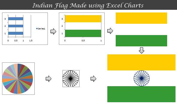
See the example Indian Flag I have constructed:

As you can guess, Indian Flag is a bar chart with 3 bars and a 24 sliced pie chart in the middle.
(There is a minor error in the chart, the spokes of the Ashoka Chakra – the wheel in the middle are not lines, but more complex. But from Flag Project perspective, that is kind of OK. More on Indian flag symbols & design.)
Here is a de-construction of the Indian flag Excel Chart:
[click here to download the Indian Flag – Excel Chart source file]
Now it is your turn,
Go ahead and make your own country’s flag in Excel using only excel charts. You can learn some powerful charting concepts while trying this. Plus, it is fun.
Follow these simple rules,
- Don’t violate your country’s flag code. Make sure you adhere to color codes, dimensions, symbol codes of your flag when making it.
- Upload your flag as an image to a free image hosting site like flickr or skydrive (upload source excel files too if possible).
- Share the url (s) of your flag image with all of us using comments.
- Feel free to make your city / town / state / book club flags as well. Share them using comments.
All the best. 🙂
PS: Due to a small visa emergency I am going to India for few weeks. The internet access back home is a bit rustic. So I will not be able to write as often as I would like to.
PPS: For inspiration and ideas on excel charts visit Excel Combo Charts | Excel Charts sections of PHD & Peltier’s Excel Charts Pages.


43 Responses
Czech Republic flag 🙂
http://wormscesky.cz/struzak/download/temp/flag.png
http://wormscesky.cz/struzak/download/temp/flag.xlsx
I don’t know why, but the chart is displayed correctly only with Excel 2007 or 2010.
I finished the American flag and should have it on my blog shortly. I must say it was very instructive, given my lack of charting experience. The stars didn’t quite come out right, I’m sure someone with Excel 2007 could produce something better looking.
Hi everybody!
We are finished the Venezuelan flag.
Here are links for the original picture and our work in MS Excel:
Original Pictures:
http://excellentias.com/wp-content/uploads/2010/03/Venezuelan-Flag.jpg
http://www.flickr.com/photos/alanz/3248934242/
Ms Excel Archive:
http://excellentias.com/wp-content/uploads/2010/03/Venezuelan-Flag.zip
Nice project!
Greetings
Here is my attempt at making the Canadian Flag. The maple leaf was a real challenge. I used 1 bar graph for the background and 3 radar graphs to form the maple leaf.
Sorry the link didn’t show up in my last post.
Chandoo:
Great idea!
Here’s my take on the USA flag:
http://www.excelhero.com/blog/workbooks/USA_Flag_excelhero.com.xlsx
It’s proportioned to the official specs at wikipedia and uses those specs in the formulas that form the chart series data.
Here’s an image for those without Excel 2007:
http://www.excelhero.com/blog/images/USA_Flag_excelhero.com.png
Regards,
Daniel Ferry
excelhero.com/blog
This is good fun. I am an Indian living in UAE so I tried my hand at creating the UAE flag and managed to do it. Can you please tell me where I can upload the file ?
Regards,
Ninad.
@Ninad: Pls. upload the file to skydrive.live.com or flickr.com (only images) and share the url here thru comments.
@All: good work everyone 🙂
Btw, if your flag has some special symbols like dragon etc, import the symbol as an image to excel and then add it to the chart instead of trying to draw the dragon 🙂
I had it pretty easy with the England flag but was fun none the less. I will upload the file to skydrive tonight. Might also try the Union Jack if I get time.
Myles
Here is the path to my file:
http://cid-4702efbc51549018.skydrive.live.com/self.aspx/Chandoo%20Forum/VBA%20Dynamic%20range%20based%20on%20value.xls
@Clarity-
Your link goes to a different Excel file, not the flag.
Regards,
Daniel Ferry
excelhero.com/blog
Reference to my post above, find the link. It’s the first time I am using this method to upload, so I hope it works, else will seek assistance
As Robert Bruce said. – “If at first you don’t succeed, try again.”
http://cid-ef586da077d21a56.skydrive.live.com/self.aspx/.Public/UAE%20flag.xlsx
Sorry here is the correct link:
http://cid-4702efbc51549018.skydrive.live.com/self.aspx/Chandoo%20Forum/England%20Flag.xls
This is funny. A couple of weeks ago I accidentally created a bar chart in a dashboard that looked like “my” flag (without the thing in the middle…)
http://en.wikipedia.org/wiki/Flag_of_the_Republic_of_Jamtland
http://en.wikipedia.org/wiki/Republic_of_Jamtland
Interesting one. Luckily, I live in a country which has a tricolour as the national flag, so no fancy stars, wheels, dragons or any other symbols required, just a simple column chart.
So, just in time for Saint Patrick’s Day, here’s the link to my flag of the Republic of Ireland:
http://cid-c7a52fb3a132adc1.skydrive.live.com/self.aspx/.Public/Irish%20Flag%20-%20The%20Q47.xlsx
Chandoo, I checked the textile colors of the India Flag:
http://en.wikipedia.org/wiki/File:Flag_of_India.svg
http://india.gov.in/myindia/images/flag1.gif
The colors are as follows:
Bar: Textile color / Pantone® / Hex / RGB
Up: Deep Saffron / 1495c / #FF9933 / 255 153 63
Middle: Dull White / 1c / #FFFFFF / 255 255 255
Down: India Green / 362c / #138808 / 19 136 8
The color of the Ashoka dharma Chakra symbol:
Navy Blue / 2755c / #000080 / 0 0 128
You used hex values: #FFCC00 / #FFFFFF / #339933 / 002060
Could you fix it?
@Pedro: Good info. I took the color RGBs from this site : http://www.crwflags.com/fotw/flags/in.html
But we can easily modify the colors. Feel free to make the changes and upload new image somewhere and share the url here 🙂
I picked up the capote (red cape in Spain) that you threw me and here is the Indian Flag revisited:
http://cid-6b219f16da7128e3.skydrive.live.com/self.aspx/.Public/flag-project-Indian2-flag.xlsx
I’ve used png archive because colors are preserved better than jpg or gif format:
http://cid-6b219f16da7128e3.skydrive.live.com/self.aspx/.Public/flag-project-Indian2-flag.png
@ Daniel Ferry – your flag design is awesome – however I was puzzled with something – how did you get a star shape thru the bubble shape…i tried to see what you did but could not figure it out…any help would be appreciated…
@Ubique: To do that, first draw the star shape using “drawing tools”. Then, select the star, press CTRL+C. Now, go back to the bubble chart, select any bubble series, press CTRL+V. Excel will replace bubbles with stars.
@Pedro: Very good work sir, very good work 🙂
@Ubique72-
I’m glad you liked it.
It’s actually very simple and the same technique works for both bubble and xy (scatter) charts. But with bubble charts you have the advantage of the star sizing proportionately.
Just insert a shape from the Insert menu. Format it the way you want. Lastly copy it to the clipboard and click on a data point on the chart for the series you are interested in and paste it. If you selected the whole series the shape will be used for the whole series. If you clicked a second time and selected just one point, the shape will be used for just that point.
You can use this technique to use images as well.
Regards,
Daniel Ferry
excelhero.com/blog
Aussie Flag. Proportions are just a guess. Stars are radar charts (at last, i have found a use for radar charts!)
http://workspace.office.live.com/?id=pACRhYmQwOWQ5MC0yOWZjLTQ4MDAtYjgyMi0wODZkN2Y1MmJkNWQAe2VmpJiVcGhHkSLsQAS7ny19ACBlZmVycmVyb0BhbmdsaWNhbmJyaXNiYW5lLm9yZy5hdQAAABTAIAsiYmN1yGZ0fgXv2_2TPVeoNAAA&cid=40
My Spanish Flag version here
http://cid-6b219f16da7128e3.skydrive.live.com/self.aspx/.Public/Spanish-Flag-pedrowave.xls
The coat of arms is from Wikipedia but is optional
http://cid-6b219f16da7128e3.skydrive.live.com/self.aspx/.Public/Spanish-Flag-pedrowave.png
Best regards.
As I like this flags exercise and as I am european, I just upload it here.
http://cid-6b219f16da7128e3.skydrive.live.com/self.aspx/.Public/European-Flag-pedrowave.png
I tried to respect the flag proportions and stars are made with a radar chart.
http://cid-6b219f16da7128e3.skydrive.live.com/self.aspx/.Public/European-Flag-pedrowave.xls
As a dream, I was playing with the transparency of stars.
Chandoo:
Here’s 42 European flags in ONE CHART!
I incorporated the flag plotting into a Eurovision 2009 project I was doing.
The Union Jack of Great Britain was the most difficult flag to plot. But many of the others are very interesting. I took great care to ensure that all flags are properly dimensioned, scaled, and colored, according to wikipedia and other sources.
Here’s a link to my post about it and the workbook:
http://www.excelhero.com/blog/workbooks/EuroVision_excelhero.com.xlsb
Regards,
Daniel Ferry
excelhero.com/blog
Sorry, that was the direct link to the workbook.
Here’s a link to the post:
http://www.excelhero.com/blog/
Regards,
Daniel Ferry
excelhero.com/blog
@Ed: Your chart is not accessible. Can you share the live spaces file with all of us (make it public).
@Pedro and Daniel: Excellent work. Thank you so much for carrying the flag forward 😉
Hi Chandoo,
I think the link works. You need to click on OzFlag (this renders the worksheet on the browser, chart is messed up), then click the Save As button to open the xlsx.
The flag was created in Excel 2010. XL 2003 would have been a better choice.
Hi
Indian flag has been explored by the key holder himself. I decided to look up any solid geometry flags.
Turkey was interesting due to its crescent (and the fact that wiki points to a 700 nano meters flag of Turkey)
Its been fun creating it in ’07, especially the crescent and star set – Ive used bubble charts for the same
Deviation from desired structure (if any) could be due to –
1. Bubble charts – its difficult to use the same scale on x, y axis and the bubbles (they seem to have a mind of their own) ; may be Chandoo can give a few pointers here
2. Angle of the star on the flag – had to do that manually no guidelines on wiki or any other site
Even though Daniel has conquered the European Union, heres my take on it
(& I couldn’t resist sharing it)
Lavkesh
links
jpg flag created
http://www.flickr.com/photos/47177133@N03/4469803785/
File saved as a 97-03 format
http://rapidshare.com/files/369222093/Flag_Project_Turkey.xls.html
Hi,
If you have please send it again?
Because of this link is broken.
Thanks
Great work, Iavkesh!
Hi Chandoo,
I just saw, that a little part of Europe is missing -> Switzerland,
so here we are:
http://www.bilder-hochladen.net/files/awnb-j-jpg.html
Out of that version, the flags of Austria, Danemark, Indonesia and
Peru can easy be done .. 😉
Kind regards,
Mike
Third time is a charm…I hope. I noticed that the url didn’t show up in my second post. Here is my Canadian flag, again.
http://www.flickr.com/photos/midnightrambler/4417610725/
Hi All
What a brilliant website Chandoo! And a brilliant flag challenge. It is a bit of a late entry, as I came across this website just yesterday. So here is my version flag of Uzbekistan. http://cid-affe60d5ed23bc13.office.live.com/browse.aspx/Public?uc=1 To view it click on Open in Excel option, Edit in Browser option messes up the file 🙁
Here is Flickr link: http://flic.kr/p/8FbK3t
The colours and size are from the flag that is displayed at Wikipedia. I used PS to get RGB values. The flag is made up from 4 charts:
Thick stripes, thin stripes – bar chart
Moon crescent and 12 stars – scatter chart.
My fiancée said that it is a bit of cheating as I am just pasting those stars in, rather than making Excel to chart it based on some formula. Hmmm, good challenge! I will try to come back with a new version…hopefully very soon!
Tokhir
Hi Chandoo, I’m new to this blog and I think I am in love! Your blog truly helped me being awesome in office 🙂
And here’s a Taiwanese flag I made with Excel. You’re right, it’s so much fun!
png: http://sdrv.ms/TAYuA9
xlsx: http://sdrv.ms/NzdGK1
http://en.wikipedia.org/wiki/Flag_of_the_Republic_of_China
Stephanie
Hi Chandoo,
I have created The Union Jack, UK flag in Excel and shared on my blog: http://eexcel.co.uk/2012/09/01/union-jack-created-excel/
using only charts 🙂
Regards, Jacek