

 Blank rows or Blank cells is a problem we all inherit one time or another. This is very common when you try to import data from somewhere else (like a text file or a CSV file). Today we will learn a very simple trick to delete blank rows from excel spreadsheets.
- Select your data
- Press F5
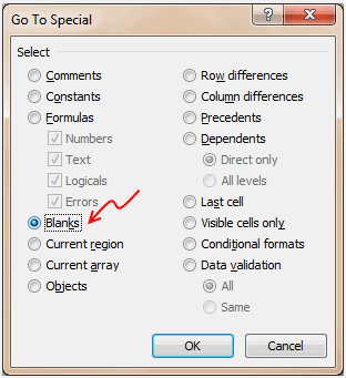
This opens “Go to” dialog in Excel. Now hit on that “select” button. - From “select special” screen, select “Blanks” (shown aside)
Now, all the blank cells will be selected. - Just press CTRL and Minus sign (-)
- Select “shift cells up” or “entire row” as needed.
That is all. Now you have successfully removed blank rows.
Bonus tip:
If you are looking for keyboard short-cut for this, here it is. Press them in the same order once you select the cells.
- F5 ALT+s k Enter CTRL+ – u Enter
Remove Blank Rows in Excel – Video
Here is a short video showing this in action. Watch closely and get rid of those annoying blank cells.


132 Responses
I was doing this with VBA, but this one is much easier and faster.
There is one thing you should be careful about. If there are some missing values in whichever column they will be deleted as well so the data will displace and probably would not match with another column(s).
Is there a way to avoid the displacement you mentioned? Such as a feature to select the rows that are empty across?
Yes. Add filters to the columns. Order the column desired and you will have the blanks at top. Delete them. Voilà!
Surprised, this works exactly the same in Mac Office 2008. Even the keystrokes are the same. Unbelievable. Thanks.
Another great tip, so simple. When I saw it, I thought “I bet that only works in 2007” but it is exactly the same in 2003. You learn something every day.
and in 2010
Check out the VBA (Macro) approach from Chip Pearson
http://www.cpearson.com/Excel/deleting.htm#DeleteBlankRows
Copy/paste into module in your personal.xls workbook and make always available when working with Excel
I use this all day long
Regards,
w
Another way to select all the blank cells is to press Ctrl+F; delete all the text, if any, in the “Find what” field; press Alt+i (or click Find All), then press Ctr+A, and then press the Esc key (or click the Close button)… all the empty cells will now be selected… follow the remainder of the instructions from the blog.
Thanks for this, I tried this method because the one above didnt work as I was using data that had been copied and paste value. The above method was not recognising the empty cells as blanks. Your method was able to identify the all empty cells and I was able to delete them.
I agree with Steve that the above method didn’t work for my pasted data. Your method worked.
This way is much better, thank you.
Thanks PHD for this and other posts….helping make us take small steps to becoming excel mini-Gurus at our work places! Will certainly share this…
Now, how do you find and delete the cells that return the null string (“”)?
This is a nice trick, but I’m too old to remember function keys and ctrl minus key combinations. So, I created another way by making a custom toolbar. By creating a custom toolbar with icons that activate these same commands.
I use Excel 2007 so these instructions only apply to that version. PHD can cover this in more detail (he probably already has).
To create a custom toolbar click on the Excel ball in the upper left side of the menu. Click the Excel Options button in the lower right side of the dialog box. Then click Customize (the 5th item down the menu list). No you have the available options for adding to your custom menu.
Change the Choose Commands from drop down list to “All Commands” then scroll down to the “Delete Sheet Rows” and add it to the list. Continue scrolling down till you find “Go To Special…..” and add that. Hit the OK button. You should now have a customized toolbar at your disposal to invoke the same commands PHD did with function keys and ctrl minus key combinations.
I do a lot of work with large tables that contain gaps. This is a very nice little trick Chandoo. Thanks for posting it.
@Cornelius: Yes, we should be careful when deleting cells / rows using this method.
@Harvey: Thanks, I didnt know Mac Excel had such good compatibility.
@Glen: Thanks for the compliments. Also thanks for blogging about this and linking 🙂
@Winston: good one, thanks for the pointer
@Rick: That is a good find (pun intended).
@Boscom: I am glad you like this…
@John: You can use “Find” to find all the values that are empty (even if they are results of formulas). Select the cells, Press CTRL+F, clear any find text, click on “options” and select “look in values”. Just hit “Find all”. Now excel finds all cells that have empty values. Now, select all the matches from find list (use shift to select) and then close the find box. Delete the cells using CTRL+-
@Dan: Good idea to use Quick Access Toolbar to launch Go to Special.
Brilliant explanation Chandoo. All the other suggestions were not working as i had values in the cells. I appreciate all the other ideas which led to your explanation. Thanks
@Chandoo and John
In Chandoo’s comment to John about selecting empty strings, his advice after clicking the “Find All” button was “Now, select all the matches from find list (use shift to select)”… you do not have to do the selections one-at-a-time… you can select all the found cells all at once by pressing Ctrl+A.
As Cornelius warns, Chandoo’s method works only if the non-blank rows are completely filled (that is, there are no blank cells in the rows that have data in them). I would also note that cells with formulas evaluating to the empty string are considered non-blank and will not be deleted; so, like Cornelius’ warning, these cells will not be deleted while the blank (non-formula) cells next to them will. With these warnings in mind, and for those who are interested in such things, the VB equivalent to Chandoo’s method is a simple one-liner…
Sub DeleteTheBlankRows()
Cells.SpecialCells(xlCellTypeBlanks).Delete xlUp
End Sub
@Winston… I think the following, much shorter, macro does the same thing as Chip Pearson’s code does…
.
Sub DeleteBlankRows()
Dim X As Long, U As Range
On Error Resume Next
Application.ScreenUpdating = False
Application.Calculation = xlCalculationManual
With ActiveSheet
For X = 1 To .UsedRange.Rows.Count
If .UsedRange.Rows(X).SpecialCells(xlCellTypeBlanks). _
Count = .UsedRange.Columns.Count Then
If U Is Nothing Then
Set U = Rows(X)
Else
Set U = Union(U, Rows(X))
End If
If U.Areas.Count > 100 Then
U.Delete xlShiftUp
Set U = Nothing
End If
End If
Next
End With
U.Delete xlUp
Application.ScreenUpdating = True
Application.Calculation = xlCalculationAutomatic
End Sub
@Winston… I copied the wrong code in my previous post; there is a single line that is not correct, but I am posting all the code to make it easier to copy/paste it…
.
Sub DeleteBlankRows()
Dim X As Long, U As Range
On Error Resume Next
Application.ScreenUpdating = False
Application.Calculation = xlCalculationManual
With ActiveSheet
For X = 1 To .UsedRange.Rows.Count
If .UsedRange.Rows(X).SpecialCells(xlCellTypeBlanks). _
Count = .UsedRange.Columns.Count Then
If U Is Nothing Then
Set U = Rows(X)
Else
Set U = Union(U, Rows(X))
End If
If U.Areas.Count > 100 Then
U.Delete xlShiftUp
Set U = Nothing
End If
End If
Next
End With
If Not U Is Nothing Then U.Delete xlShiftUp
Application.ScreenUpdating = True
Application.Calculation = xlCalculationAutomatic
End Sub
I’ve noticed that if you have merged cells then the VBA will remove some of those lines. e.g. I had an area where the A:B was merged along with C:D. If I ran the code without unmerging them fiorst then these rows were also removed. If I unmerged either of the A:B or C:D then the code did NOT affect / remove those rows.
When I want to remove blank rows of data. I just select the data and press sort Z>A. What are the limitations of that way?
@Wendell… That will work, of course, but it does have the side effect of leaving the data “out of order” which may or may not be a problem. If the existing data is in order with internal blank lines, then if there is a naturally sequential column (such as an “data entered date” or sequential “order number”), the data can be resorted on this column to put the data back into its original order. Otherwise, you can create a sequentially indexed column, sort the data Z-to-A according to one of the existing columns, delete the index numbers next to the blank rows them, and then sort the data A-to-Z on the index column to put the data back in the original order; but, of course, this involves (a small amount of) extra work to do.
@Rick… awesome discussion, thanks for your knowledge and passion. 🙂
I have been inserting a column and using edit, fill, series to get sequence numbers. Then sorting on the column containing blanks and deleting rows. It is quite fast but Chandoo’s idea sounds simpler.
When I know I am going to do a lot of crazy sorting I sometimes add a sequence column just to get back to my original order.
Many great tips – thank you!
Always Brilliant,but be careful about deleting some needed data as
Cornelius commented
Regards
This Tip is awesome.. 🙂
Amazing!!! Thank you so very much!!!
Nice..
To Rick Rothstein (MVP – Excel):
This was the perfect trick for what I needed to do. Thanks
@Jared,
I presume you are referring to my method of selecting all the blank cells… you are quite welcome… I am glad you were able to make use of it.
This is very helpful, but on my Mac with Excel 2008, it crashes (wheel spinning and “not responding” on Force Quit) every time I hit the control-. I am trying to delete blanks in columns of data that are a couple of thousand rows long though!
I tried this method but excel can’t seem to find an of the blank cells in the range i selected. There is nothing in them but when i click on them and then press delete, excel can find them. This defeats the purpose of the go to method because i have to click on every cell individually. Anyone have any ideas?
Hi this method helped me. Thanks a lot!
Great information. I could not get it to work at first. It took me a long time to figure out even though my cells were blank, they had some sort of value when I imported the file.
So I copied all the cells then pasted as text into another spreadsheet. Then i was able to select all the blank cells and move everything over to the left.
This is not working for me. The rows are still there. Just blank now. CRTL x, CTRL -, nothing works.
Thanks.
This worked perfectly and saved me a lot of work in both looking for a solution and performing the work!
coooooooooooool saved me a LOT OF WORK
thanks again!
Worked great. Many thanks.
Certainly saved a lot of time for me!
Thought about trying to figure this out by myself then thought it would be a waste of time if someone already figured it out for me. Appreciate you taking the time to post this so we could glean from you!
Thanks for the demo, this was very helpful. This is certainly a time saver tip. 🙂 I appreciate it.
This work great, thanks for good example. I tried to find the way to remove empty cell like this and your tip is great. Thank you.
Thank you soooooooooo much worked, just have to qc the data to see if the values were copied correctly.
thanks again
I should stop Googling questions about Excel and just head straight to Chandoo.org!
Thanks, You rock!!!
thanks you saved my day and time
I follow the steps, and it works. Wonderful tip!
But i wonder if there is a faster way to delete all the blank rows or not, and then i found that some excel applications can deal with this issue with only one click. The one I try now is Kutools for Excel, it is an excel add-ins collection and provides a function to delete all empty rows just by clicking on the function button. Very simple to use.
Include but not limit to the delete blank rows function, Kutools for Excel can help deal with some repetitive work, such as rename multiple sheets, sort sheets , and so on.
@Evelynmorry
There are a number of tools which do exactly that
You should inform readers that you work for ExtendOffice or risk ending up in the spam bin.
Thank you, appreciate the clearly written directions.
haha…
this is cool 😀
Thanks for sharing mate 😉
Thanks so much!! this is a great help.
I had done a row deleting the blanks manually which really waste time.
This can be done in mere seconds 🙂
Thanks a lot!!!!! 🙂
Thanks so much!!!!!!!!!! It’s been really really useful!!
Thanks! it worked 🙂
This was an awsome tip! Can’t get nearly as good help from Microsoft’s help menu!
Thanks mate, you just saved me from deleting so many cells!!!
simple but productive tip… 🙂
I have read many of these comments, I tried deleting with this method, but I only want to delete blank rows – not blank cells. As stated we must be careful all the data shifted up and was not readable. I used to know a way to delete only blank rows and can’t remember now. I will come back for more tips that may help in other areas. Thanks
Hi
The post is helpful. However, I need to delete empty rows from multiple worksheet in a single file. I would have done it manually if I had one excel file. However, I have around 200 excel files with almost 100 sheets in a file. I appreciate if anyone could help me with VB code or a general way to save time.
Maybe i’m confused, but why wouldn’t you just custom “sort” them out instead of deleting or going through all those steps? I can understand if you want to remove/delete blank cells, but that messes with the data when there are values surrounding the blank cell. To “remove” (put blank rows at the bottow), couldn’t you just use a custom sort?
All this information here is very valuable, but some are overkill for the topic at hand… aren’t they? Maybe it is just me.
Good luck with your data crunching!
Thanks a lot
Nice tips! There’s always a way out of every challenge, either in Excel or in the real world. Thanks a lot!
Thank you so much….it has proven to be of great help.
YES! You saved my day! I was afraid I had to delte 1500 blank cells my self.
Your karma has improved today 🙂
Thanks a lot… it was a great help
Fantastic! Very simple (and correct!) instructions. Thank you!
Thank you, Chandoo! You’re a genius! 🙂
awesome…. thank you so much. It saved lot of my time
Thank you 😀
Its not working for me. Is there a key you have to hit f5 with after you’ve highlighted the data?
I just needed to delete a bunch of blank rows and found this site. Some of my filled in rows had one or two empty cells causing the problem of losing rows I actually needed.
I found a fix. Instead of just hitting F5 so that the whole worksheet is selected click on one of the columns and then do F5 and select blanks. This results in only blanks in that column being selected. Then ctrl – and delete row works. Just have to have at least 1 column that is completely full
Thanks !! a lot , This is very useful formula for excel users
Very useful. Thank you. 🙂
Hey Bro,
Thank you very much,,
very use ful for me.. You have given the info very cleary.
One limitation I found was that if you have a formula such as “=if(a1=1,true,””)” in a cell, then paste values, if the formula previously resulted in “”, excel does not consider that cell blank. I was having difficult deleting these cells.
The roundabout way i found around this was to conditional format the entire group of cells with any CF, then “Go To – Special – column differences” and clear rules from selected cells. Then “Go To – Special – Conditional format” and you should have your “blank” cells.
Works a treat, thank you very much for blogging this! 😀
Awesome dudeee. Saved me an hour work 🙂
Awesome tip. Saved a lot of time, thanks a lot.
i want to Delete a row by comparing two cells,if two cells are blank then delete that entire row.
You just saved me a shitload of work mate thank you!
Great help! Saved me tonnes of time. Was faffing with filters before!
Thank you!!!
What an awesome thing to know — this will save me a lot of time!
Tip is awesome!!Thanks for sharing..
Hi all, i’m doing this “blankcellminator” but my data is just to big
any idea how to do the “blankcellminator”? besides manually selected the area?
Excellent !!! THank you verymuch for publishing this… I had been struggling with this from long time.
Thanks for sharing the useful info..
BRILLIANT!!! Thank you so much!
Great Tip. Thanks
Guys, hard problem, need help
I must report all the cells from a previous sheet that respect a particular condition, otherwise consider the cell like blank. the problem is that this must be automatic, in the sense that i need that this operation devolps every time with different records sheet. the problem is that excel, in the second sheet, consider the blank cells which are the result of the conditional formulas non like blank cells, and in fact when i try to order the numbers obtained like result, excel orders the blank cells before the numeric cells. I can not delete the formulas in the blank cells because it must be able to operate with different sheet record time after time (lenght can vary).
question: How i can get blank cells like result from a formula that are considered not like number by excel and therefore ordered after numeric cells if sorted?
@Dave
How about asking this question in the Forums
http://chandoo.org/forums/
.
It may be helpful if you post a sample file:
http://chandoo.org/forums/topic/posting-a-sample-workbook
Very helpfull, thanks a lot. If I have to delete all rows with “John” in it. Do you know how to do it? Thank you
The Problem I see with several versions of Excel, but especially 2010 and above: Excel somehow places thousands of cells in range. I have data in columns A:F, but if I select all (A1 + Ctl+Shft+Down), it takes me over as far as column WWW. This is so many cells that Excel freezes and I have to restart. I need a way to delete those blank columns that does not upset Excel. Anyone else have that problem?
Thank you very much.
Chandoo – thank you, thank you, thank you! I have just had to redo a whole heap of data analysis, due to a botched custom sort, this has saved me a truck-load of tedium – your a star!
super helpful! saved me so much time!
Thanks you are a genius.. 🙂
This is awesome. Thanks so much.
Ned
Hi Chendoo,
Your post is a very good piece of information.
However, could you please help me with another issue?
In Excel 2007 I have made a macro selecting the entire column. The selection has written information in 65000 rows (the file was saved at that time using Excel 2003). Regardless of my erasing the data from the rows 1000 to 65000, the cells remain “active” somehow, and that makes the file huge. Unfortunately I can not CUT and PASTE the information in another sheet due to the fact that I have a lot of formulae linked to the information from this sheet.
Do you have an idea on how I can get rid of the unused rows?
Thank you!
Aurelia
Aurelia
Can you simply select the rows 1000:65000 and delete them?
Also have a read of the comments here:
http://www.msofficegurus.in/2011/03/compress-excel-workbooksreduce-file-size/
+
http://stackoverflow.com/questions/3003349/reduce-the-file-size-of-excel
+
http://datapigtechnologies.com/blog/index.php/how-to-compress-xlsx-files-to-the-smallest-possible-size/
Make sure you have a backup of your file to start with
Hi Hui,
Thank you very much for your reply.
It did work with selecting and deleting the rows, but the result (the decrease in file’s size) was visible only after saving the file. 🙂
Also, thank you very much for the links, as they are extremely useful for what I am doing right now.
All the best,
Aurelia
@Aurelia
Thats great news
Yes, the File will only change size when it is re-saved
Until it is saved you can cancel any and all changes by not saving it
YEAH! Different ver of Excel but worked WONDERFUL! THANK YOU!
Superb Tip!! Made life easier in a Jiffy. Thanks a lot
Thanks very much for this , made my job easier:) I’m glad i’m the 100th commenter 🙂
Not sure if anyone’s mentioned this method, it uses the “Sort Z->A” method without (ultimately) breaking the order:
1. In the column next to the data column (including blanks), type “1”, “2”, select those two cells, and then fill the remaining cells in the column for the data (drag the corner down to the end of the data), so that it fills the column with 1, 2, 3, 4, …
2. Select the data column, sort reverse-alphabetically from Z->A (when asked, “Expand the selection”), thus placing the empty data rows below the filled data rows (but breaking the order).
3. Either delete the blank data rows or copy the filled data rows (including the numbered column) to another sheet.
4. Select the numbered column, sort from smallest to largest (when asked, “Expand the selection”), thus restoring the original order.
5. Delete the numbered column.
This approach is good and quick (and I don’t think it cares about whether a cell is truly empty or not) as long as you don’t mind navigating to the end of the data.
Thanks a ton!!
thanks man… good job!
AWESOME!! Thank you.
thanks .
thanks cuhh
Nice one ….this one worked at the first attempt. Great. Thank You
Thank you!! This saved me so much time and made me look like such a smart ass ” work. I love you forever.
at work *
misspell sorry
i just wanted to check if above technique can be used to delete only blank rows..
Column A Column B Column C
1 add A
2 Sub S
3 D
4 Mul M
5 Mod
6 Abs As
8 Avg Ag
Please note, in the above table, Cell B3 is empty, but the complete row is not empty. Similarly, C5 is empty, but not the complete row. But row 7 is completely empty. In my excel, there are many such empty rows, and in between there are some cells which are empty too… so if i use F5->special->Blanks… excel selects all blank rows and also the cells… But i wanted to delete only the blank rows, and keep the empty cells as is.. because some of the other columns in those row are valid… so how to delete only fully blank rows…
Good one !
Thanks ! its work for me !
https://69d6a2dd5579e63ca4b7019c81e270f8113310f6-www.googledrive.com/host/0B7a8lPjWeTRzZW93Q1R4VzdjbVE
i love u
Thanks Chandoo. Saved lots of time.
One question: what is the difference between shift cells up ft cells up” & “entire row” ?
I only ask because when i used entire row the result is what not i expected
Thanks!!
Wonderful! Your hint helped me a lot! Thanks! 🙂
How can this be done in LibreOffice?
@Philip
I’d ask the question in a LibreOffice Forum