
Steven, one of our readers from England sent me a Christmas gift tracker worksheet. I found it pretty cool, so made some minor changes to it and am sharing it with you all so that you can have great time shopping for the holidays.
Why I found this Christmas Gift List Spreadsheet Cool?
There are probably a million other gift trackers out there, but I liked Steven’s version for few reasons:
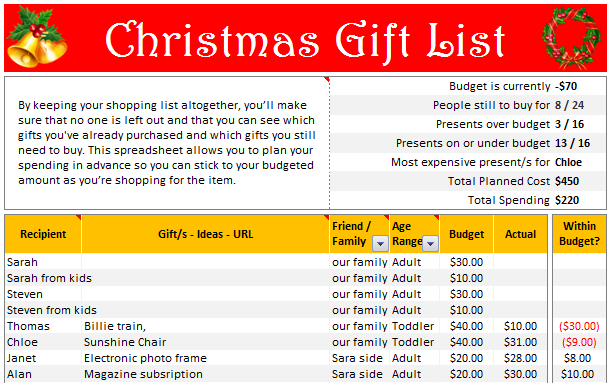
- He used conditional formatting to zebra line the gift-table.
- He used array formulas to find-out who is receiving the most expensive gift. The formula relies on VLOOKUP coupled with SUBTOTAL so that when you filter the list to see gifts only for certain age group, the formula shows most expensive gift receiver in that group alone. How cool is that 😎
- He used cell formatting to highlight gifts overshooting budget in RED color.
- He used SUMPRODUCT liberally to summarize the gift data to show us “how many people got the gifts”, “how many gifts are over the budget”, “how many gifts are under-budget”.
Go ahead and download the workbook. Even if you dont have a huge list of gifts to buy this Christmas (REALLY ?!? You dont have a long list? Can I please, please get that wii?). The workbook is full of excel lessons on conditional formatting, formulas and design.
Download the Christmas Gift List Spreadsheet
Click here to download the file. It is protected to make sure you accidentally erase a formula or something. But there is no password. So go ahead and unlock it to learn something cool.
Thank you Steven,
for your most thoughtful and awesome Christmas gift to our community.


15 Responses
I’m confused: if you spend $10, and your budget is $40, shouldn’t the amount in the “Within Budget?” column stay black, since you didn’t go over budget?
In other words, since we overspent on the electronic photo frame, shouldn’t the $8 cell turn red?
@JP.. maybe Steven is encouraging consumerism… ?
I havent realized it earlier, but now I see it. If you unprotect the sheet, you can change the formula in Column I to =IF(G13=0;” “;F13-G13) from =IF(G13=0;” “;G13-F13), that should correct the behavior.
Thanks Chandoo. I thought of making a shopping list spreadsheet for Christmas, but this is neat so I think I’ll use this instead.
Chandoo & Steven thanks for this spreadsheet. But for the sake of a person who has been staring at this megaformula in vain for the last 40 mins and not afraid to ask, would it be possible for you to walk us through the logic used here?
=SUM(SUMPRODUCT(SUBTOTAL(3,OFFSET($K$13:$K$62,ROW($K$13:$K$62)-MIN(ROW($K$13:$K$62)),0,1)),–($K$13:$K$62=”-“))+SUMPRODUCT(SUBTOTAL(3,OFFSET($K$13:$K$62,ROW($K$13:$K$62)-MIN(ROW($K$13:$K$62)),0,1)),–($K$13:$K$62=”0″)))&” / “&SUBTOTAL(2,$G$13:$G$62)
Thanks Chandoo.. This is one of the best budget spreadsheets I’ve ever seen.. The Arrays are out of this world!! And it’s FREE!!
Chandoo, can you tell us more about Steven? Does he have his own site?
JP, I think Chandoo changed it when he changed the currency formatting from £ to $, a negative figure is a good thing in this case. But don’t change the formulas, the overbudget and under budget won’t work properly if you do. Also Chandoo I think you’ve accidentally broke the conditional formatting for the alternating row colouring the formula is different to the version I sent you. As for the megaformula chrisham, it gave me a headache trying to get it all working, so I will let Chandoo talk you through it.
Hi,
In cells I6 and I7, I understand that subtotal together with offset function returns an array of ones after which, the sumproduct function gives the desired result.
But I’m not able to figure out the reason for using an array in I8 to return the most expensive gift.
Can’t the formula be just
“=VLOOKUP(SUBTOTAL(4,$G$13:$G$62),$G$13:$J$62,4,0)”
Savithri, Cell I8 needs the array, if the formula was “=VLOOKUP(SUBTOTAL(4,$G$13:$G$62),$G$13:$J$62,4,0)” it would find the highest price from the filtered range (i.e. highest actual in filtered range is $50) BUT then return the first person with that actual, not looking in just the filtered range (so first person on the list with a $50 actual.)
To see what I mean, change the formula, then change all the actuals to $50 then filter for baby, it lists the first name on the list.
But a good question 🙂
Thank you. I now realise that the array is used to get the ‘filtered range’ instead of the entire range, as table array for look up value.
this looks like an awesome excel sheet!! is there anyway i can get it emailed to me unprotected? for some reason, i am unable to download it 🙁 help!!
Hi I also can not download to a mac as the sheet is protected any help would be great