
 Most of us think of mastering formulas, learning macros and being supergood with charts when we think of being productive with spreadsheets. But often learning simple stuff like keyboard shortcuts, using mouse and working with menus and ribbons can be a huge productivity booster for us. So as part of this installment of spreadcheats we will learn 7 very cool and effective double click tricks in excel. (as an aside, try saying double click tricks several times faster… 😉 )
Double Click on the Office Button / Logo to Close Excel
![]()
This is simple. Displays “do you want to save…” dialog if the workbook is not saved.
Adjust column widths by selecting multiple columns and double clicking on the separators
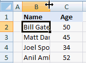
This is my favorite. You can use the same trick to adjust row heights too.
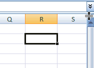
Double-click in the corner, just above scroll-bar to include a split
It is surprising that very few people know about split and freeze panes feature in excel. I have often seen colleagues struggling to freeze top row of a large workbook or include a split so that they can see 2 different things at a time.
You can also create a vertical split by clicking on the little bar shape next to horizontal scroll-bar near bottom right corner of the excel window.
(If you are wondering where the split would be created, it will be created at selected cell’s row (or column))
Double click on ribbon menu names to collapse ribbon to get more space

In MS Office 2007 you can double click on the ribbon menus to collapse the ribbon to one line. In Excel 2003, when you double click on the empty space in the toolbar area, it opens up the “customize” window (same as Menu > tools > customize)
Auto-fill a series of cells with data or formulas by just double clicking
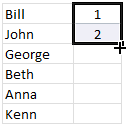
I have saved countless minutes ever since I learned this little trick. Lets say you have a table where in one column you have some data and in the next you have written a formula in the first row. Now how would you copy the formula and paste it in all cells in that column?
Copy the formula (ctrl+c), select all cells, paste the formula.
Well, no more. Just select the formula in first cell, double click in the bottom right corner and see the magic.
The trick works for formulas, auto-fills (of numbers, dates, what not) as long as the adjacent column has data.
Jump to last row / column in table with double-click

Just select any cell in the table and double click on the cell-border in the direction you want to go. See the screencast.
Lock a particular feature and reuse them with double-click

You can lock any repeatable feature (like format painter, drawing connectors, shapes etc.) by just double clicking on the icon (in Excel 2007 this works for format painter, but for drawing shapes you need to right click and select lock drawing mode). This can save you a ton of time when you need to repeat same action several times.
Now its time to test your clicking skills
Try clicking on these: excel keyboard shortcuts, excel mouse tips & tricks, excel productivity tips part 1 & part 2
ok, I am kidding, but you get the point.
What is your favorite double-click-trick?
tell me please…


