
This post builds on earlier discussion, How many hours did Johnny work? I recommend you to read that post too.
Lets say you have 2 dates (with time) in cells A1 and A2 indicating starting and ending timestamps of an activity. And you want to calculate how many workings hours the task took. Further, lets assume,
- Start date is in A1 and End date is in A2
- Work day starts at 9 AM and ends at 6PM
- and weekends are holidays
Now, if you were to calculate total number of working hours between 2 given dates, the first step would be to understand the problem thru, lets say a diagram like this:
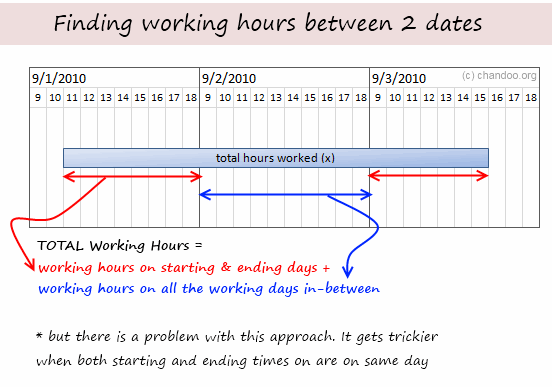
We would write a formula like this:
=(18/24-MOD(A1,1)+MOD(A2,1)-9/24)*24 + (NETWORKDAYS(A1,A2)-2)*9
See the above illustration to understand this formula.
Now, while this formula is not terribly long or ineffective, it does feel complicated.
May be we can solve the problem in a different way?!?
Michael left an interesting answer to my initial question, how many hours did Johnny work?
Pedro took the formula further with his comment.
The approach behind their formulas is simple and truly out of box.
Instead of calculating how many hours are worked, we try to calculate how many hours are not worked and then subtract this from the total working hours. Simple!
See this illustration:

So the formula becomes:
Total working hours between 2 dates – (hours not worked on starting day + hours not worked on ending day)
=NETWORKDAYS(A1,A2)*9 - (MOD(A1,1)-9/24 + 18/24 -MOD(A2,1))*24
After simplification, the formula becomes,
=NETWORKDAYS(A1,A2)*9 - (MOD(A1,1) -MOD(A2,1))*24 -9
=(NETWORKDAYS(A1,A2)-1)*9 +(MOD(A2,1)-MOD(A1,1))*24
Sixseven also posted an equally elegant formula that uses TIME function instead of MOD()
=(NETWORKDAYS(B3,C3)*9) - ((TIME(HOUR(B3),MINUTE(B3),SECOND(B3))-TIME(9,0,0))*24) - ((TIME(18,0,0)-TIME(HOUR(C3),MINUTE(C3),SECOND(C3)))*24)
Download the solution Workbook and play with it
Click here to download the solution workbook and use it to understand the formulas better.
Thanks to Pedro & Michael & Sixseven & All of you
If someone asks me what is the most valuable part of this site, I would proudly say, “the comments”. Every day, we get tens of insightful comments from around the world teaching us various important techniques, tricks and ideas.
Case in point: the comments by Michael, Pedro and Sixseven on the “how many hours…” post taught me how to think out of box to solve a tricky problem like this with an elegant, simple formula. Thank you very much Michael, Pedro, Sixseven and each and every one of you who comment. 🙂
Have a great weekend everyone.
PS: This weekend is my mom’s birthday, plus it is a minor festival in India. So I am going to eat sumptuously, party vigorously and relax carelessly. Next week is going to be big with launch of excel school 3.
PPS: While at it, you may want to sign up for excel school already. The free lesson offer will vanish on Wednesday.


5 Responses to “Preparing Profit / Loss Pivot Reports [Part 2 of 6]”
[...] Preparing Pivot Table P&L using Data sheet [...]
[...] Preparing Pivot Table P&L using Data sheet [...]
[...] Preparing Pivot Table P&L using Data sheet [...]
I am not getting sound from the videos. I have checked all the settings and spent several hours searching the Internet to no avail.
Has anyone else had this problem?
Is there anyway to get the Grand Total to be broken out in the same fashion as the items above it? For instance, if you have in column 1, widget a, widget b, and have their sales by month in column 2, I'd like to see the grand total also be by month, for widget a & b combined.
I can't get anything other than a single line for the grand total, rather than the same format as the data above.
Widget A Month Sales
Jan 100
Feb 200
Widget B
Jan 150
Feb 250
Grand total - here I would also like to have Jan, Feb.
Jan 250
Feb 450