Quickly Remove Data Validation Rules using Paste Special

Here is a quick tip on removing data validation rules.

We all know that data validation is a powerful feature in Excel to control what data is entered. But, sometimes, you may want to remove the rules from a set of cells. How would you do it?

The normal approach is,

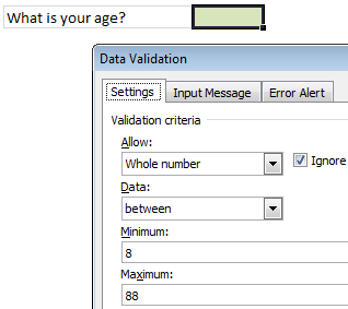
1. Select the cells with data validation rules
2. Go to Data > Data Validation
3. Select rule as “any value’
4. Press OK

In short, you have to move your mouse alot. It would make sense if we accumulate frequent flier miles on the mouse travel too.

Shouldn’t there be a shorter, quicker way?!? Well, of course, there is a way.

We use Paste Special.

What ?!? Paste Special?!?

That is right. A simple paste special can remove the data validation rules for us quickly. Here is how.

1. Select an empty cell without any data validation on it. Press CTRL+C
2. Now, go back to the cell(s) from which you want to remove data validation rules
3. Press ALT+E S N (In other words, Paste Special > Data Validation)
4. Press OK and you are done.

How does it work?

Simple, we took the data validation rules from empty cell in (1) and then pasted them over our original cell(s) using Paste Special option.

What next?

Nothing, Its almost weekend here. We are taking a train to go to a place 400 kilometers away to see a classmate and close friend getting married. Lots of fun and partying awaits. When I am back on Monday, I will surprise you with more Excel awesomeness.

Go ahead and enjoy your weekend…

PS: Paramdeep reminds me that Financial Modeling School enrollments close on March 8th – just 4 more days. Sign-up already.