
Lets say you are the head of purchasing department at Big Corp Co.
You are obviously very busy. Every day starting with a large cup of coffee and ends with a big smile, as you save your company thousands of $s by negotiating best deals, finding best providers and being awesome.
Today, let me share a small Excel tip with you that will make you even more awesome.
Finding a provider with lowest value:
Lets say you are looking at a table like below and want to find-out lowest priced providers for each service.
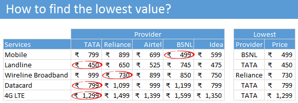
To find providers with lowest value:
- Find the least amount for each service. Assuming the services are in the range C5:G5, use =MIN(C5:G5) to get this.
- Give a name to list of providers. I call mine as providers
- Using INDEX, MATCH formulas find the provider name with lowest amount. Like this:
=INDEX(providers, MATCH(minimum_value, C5:G5, 0)) - Bingo. You have the answer.
Bonus tip #1: Highlighting lowest values.
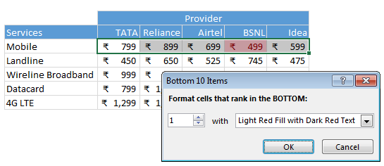
If you just want to highlight the lowest values, use conditional formatting.
- Select first row of numbers.
- Go to Home > Conditional Formatting > Top / Bottom rules > Bottom 10 items
- Set to Bottom 1 and specify formatting as you want.
- Using format painter, copy the conditional formatting, one row at a time.
- Done!
Bonus tip #2: Handling Ties
Often 2 or more providers will tie for the bottom spot. What then?
One way to handle the ties is to show the word ties when 2 or more names have lowest value. To do this, use this formula instead.
=IF(COUNTIF(C5:G5, minimum_value)>1,"Ties", INDEX(providers,MATCH(minimum_value,C5:G5,0)))
A formula challenge for you…
Now that you know how to find the lowest value, here is a challenge for you.
- How do you write a formula to find which provider has maximum lowest values. In this example, the name we are looking for is TATA as they have 3 lowest values.
Want to find more… look here:
If you want to find more Excel formula tips and techniques, look no further. Start your journey with this and see how deep your formulas can nest.


One Response to “CP034: Advanced Excel Essentials book talk with Jordan Goldmeier”
I like this book, but I'm biased