
Most of you know that during day time I work as a business analyst. Today while preparing some test scenarios for our latest insurance application, I came across a weird problem.
There are some steps in testing. For each test scenario, a combination of these steps is required. It is my responsibility to identify the steps as well as their combinations for each of the scenarios. So I quickly prepared a table with all the steps in left most column and one scenario each in one column. I put “X” in a cell if the step needs to appear in that scenario. But when I gave it to our testing team, they asked me if the scenarios can be explained a little better. See this picture to understand what they want and what I made.

So I immediately converted the “X”s to actual step names using a simple IF formula. (Copied the table, and wrote ‘if there is an X in the previous table, get the actual step from left most column otherwise empty‘).
Then the problem of actually removing various blank cells. First I tried to select all the blank cells and remove them using our technique from last week. But it failed as the blank cells are actually formulas with empty values. So I copy pasted the entire table as values (CTRL+C, ALT+ESV). But even then excel wont recognize blanks as true blanks (because the value is actually “” instead of being plain empty.)
Now I didnt want to manually select all the blank cells as the real testing scenario table had 50 scenarios with 68 possible steps.
Then it stuck me, why not use FIND (CTRL+F) to find all the cells containing nothing? So I selected the scenario table, opened the find and looked up all the cells that contain empty values. Now I clicked on “Find all” and selected the entire list of values from that. Finally I removed all these cells and bingo!
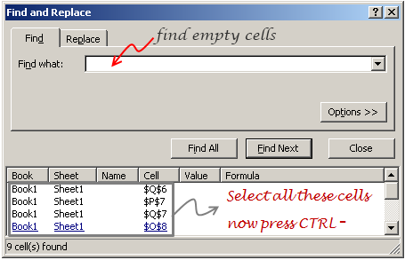
PS: Our testers was more than happy as it took very little time and they had all the scripts ready.
PPS: Thanks to Rick, who taught me FIND ALL approach to select blank cells (here).


