Quickly Fill Blank Cells in a Table [Reader Tip]

This post is authored by Martin, one of our readers.

Situation:

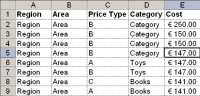
Sometimes I encounter data in my tables with blank cells where there is a repeated value from the cell directly above. See below:

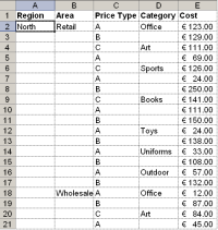
This can be annoying when it comes to interpreting the data and when sorting columns.

Solution:

Here’s the solution I use.

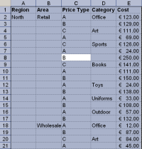
1. Select the whole table. I favor the shortcut Ctrl A to do this. Make sure you perform this shortcut from within the table though as otherwise the entire worksheet with be selected. This gives us Figure 2:

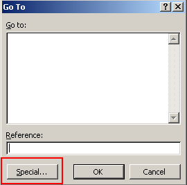
2. Next we will open the Go To dialog box. This is a very useful dialog for selecting certain types of cells, for example cells containing formulas, constant values, visible cells and so on. F5 or Ctrl G both work as keyboard shortcuts.

3. Click the Special button (see Figure 3)

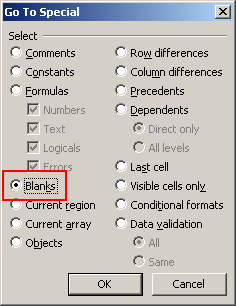
4. In the next screen select Blanks.

5. Click OK and notice that all blank cells are now highlighted in the table (Figure 5). Notice too, the position of the active cell. This is the one un-shaded cell in this selection. In this example it is cell D3. If the table were fully complete this cell would show the same value as the cell above it – cell D2 – the word Office.

6. Next we will use the fact that cell references in Excel by default behave in a relative manner. That means when you copy a formula to another cell, the cell reference in the formula change relative to the location in the worksheet it has been moved to unless they have been made absolute.

7. Without clicking any of the cells in the data, simply enter the following simple formula:

=D2

If you are following along here with a different table, then you will substitute the cell reference of the cell directly above your active cell. (Figure 6)

8. Next the important part. We need to copy this simple formula to all the other blank cells which could number in the hundreds or thousands or greater still. How do we do it?

Simply by using one of the best keyboard shortcuts I know in Excel: Ctrl & Enter.

This shortcut when used in a single cell will enter the value inputted into the cell and keep that cell active, instead of performing a carriage return to the next row.

But, when used over a range of cells, Ctrl & Enter together will copy the value of the active cell into all cells in the selection.

In this case, we are not going to copy the value of D2 into all blank cells, but the relative cell that appears over each blank cell. In cell D3’s case this was D2. In A3’s case for example it is A2 and so on.

After CTRL Entering the formula the worksheet now looks like:

9. There is one last important step. These pasted valued are, as we have seen, relative formulas. If I were to change the sort order in one of the columns, for example to identify which Cost in column E is the highest, my table would be completed distorted as the formulas in the changing rows are all retrieving the value in the cell above. See Figure 8.

I’ll Undo my flawed Sort by clicking Ctrl Z.

The final step therefore is to change these formulas into constants so that this type of problem can be avoided.

To do this, select the table, (or if the formula cells remain highlighted, you won’t need to select the table at all).

Now copy your selection with Ctrl C.

Next, perform a Paste Special / Values to replace the formulas with their constant equivalents – Figure 9.

And that’s it!

Thank you Martin

Many thanks to Martin for sharing this simple yet very beautiful trick with all of us. If you enjoyed this article, say thanks to Martin.

How do you deal with Blank Cells

Barking dogs, bad bosses and blank cells are everywhere. I am eager to know how you deal with them. Please share your tips & techniques with us using comments.

More on Blank Cells and other Unclean Data

If you constantly deal with blank cells or other types of unclean data, read these articles to learn few more tricks.

• Delete Blank Rows in Excel Tables
• Removing Blank Items in a range of cells
• Cleaning up Dates in Excel
• Merge Several Cells without Loosing Data [macros]