
Here is a 2011 new year gift to all our readers – a free 2011 calendar template.
(a little secret: just change the year in worksheet “Full” from 2011 to 2012 to get the next year’s calendar. It works all the way up to year 9999)
You can add notes to individual dates or complete month using the excel template very easily. There are 6 different calendar templates in the download file,
- 4 Yearly Calendar Templates with different color schemes.
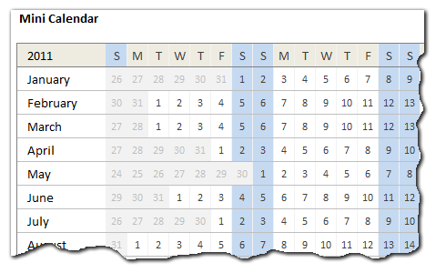
- 1 Mini Calendar
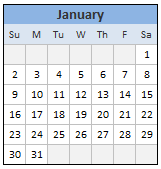
- 1 Monthly Calendar (prints in 12 pages)
![Free 2011 Calendar - Download and Print Year 2011 Calendar today - Excel Spreadsheet Template for Yearly Calendar [2011]](https://img.chandoo.org/c/2011-calendar-template-download-free.png)
Download 2011 Excel Calendar Template
Download the Printable 2011 Calendar – in PDF format
Download the 2011 Calendar Spreadsheet – Excel 2007+ | Excel 2003
More Calendars: Year 2010 Excel Calendar | Year 2009 Excel Calendar
How this Calendar works?
Read on if you are curious to know how the formulas are cooked in this calendar…,
- The cell D3 in worksheet Full has the year of calendar. I named this cell as year.
- All the formulas for the calendar are written in the worksheet mini.
- For this year’s calendar, I took inspiration from Daniel’s Live Calendar example (Recommended reading for formula enthusiasts).
- The first step to create a calendar is to generate a sequence of numbers 1 thru 42 (because calendar grid has 42 cells – 7 days per week x 6 weeks max, per month). I used a combination of INDIRECT, OFFSET and COLUMN to get this. The formula is
=COLUMN(OFFSET(INDIRECT("$A$1"),0,0,1,42))-1. I mapped this formula todaysAndWksnamed range. - Next step is to find the first date of each month using a simple date formula like
=date(year,month,1). This formula is mapped to named range –DateOfFirst - For given month, the calendar is nothing but
=daysAndWks + DateOfFirst - WEEKDAY(DateOfFirst,2). This formula is mapped to named range – calendar.
 Once the mini calendar is ready, I just created 12 named ranges m1_, m2_,…, m12_ corresponding to each of the 12 months.
- Then, I used the same in individual calendar worksheets along with INDEX formulas to fetch the dates.
- Finally, I formatted the calendars nicely. Design of this calendar is similar to that of 2010 calendar & 2009 calendar templates.
Go ahead and enjoy the download. The file is unlocked. So poke around the formulas and named ranges. Learn some Excel.
More Downloads: Download Free Excel Templates
Techniques used: INDEX | OFFSET| INDIRECT | Array Formulas | Using Date & Time in Excel


99 Responses to “How to use Date & Time values in Excel – 10 + 3 tips”
[...] Date with my sheet - 10 tips on using date / time in excel (tags: excel totw) Posted in Uncategorized | [...]
I have this current formula in place for 2014 "=DATE(YEAR(TODAY()),T2,1)"
How do I change it for 2015?
Thanks 🙂
@Liz
You shouldn't have too
If you use it today 1st Jan 2015 it will return the 1st of the month in cell T2 in 2015
[...] 10 Tips on using Date / Time in Excel [...]
[...] More on date / time: 10 tips on using, formatting date / time in excel. [...]
Hi Chandoo,
Since this article was for Dates, below are 2 easy ones to calculate the Start and End of Month. (without using the EOMONTH formula as available in Analysis Toolpak).
In Cell A1, put any date
then in the cell where you would want the Start of Month put the below formula
1. Start of the Month
=DATE(YEAR(A1),MONTH(A1),1)
2. End of Month
=DATE(YEAR(A1),MONTH(A1)+1,0)
Hope this would help a lot who were dependant of EOMONTH..
cheers
~Vijay
@Vijay: That is an awesome tip. Thank you so much for sharing it with all of us.
Perfect
Why not use the EOMONTH formula?
I run a trolley tour business and need to set up a data base to track tickets sold by mutable vendors (from store, on the street ,etc)and by class ( adult, senior,child and discounts ) can you help or direct me to one that could?
I know how to write macro's for excel, but I have 1 issue that I cant figure out and would appreciate some help.
I want to key a range of dates, (7/1/09-7/12/09) then write a macro to go find the info for that range and bring it back to my spread sheet.
Thanks for any help....
@Glenn: you can try a user defined function if the information you want to gather can be derived only from the 2 dates entered. You can write a macro, if you need to refer to other ranges in the workbook to gather the info based on the dates entered. I am not sure what you meant by "go find the info for that range". May be if you tell what you are trying to find, I can suggest the approach for writing a macro...
[...] Important excel formulas: IF and Then, Vlookup, Offset, Sumif, Countif, Working with date and time [...]
[...] Tips on using date & time in excel, List of excel date & time formulas, More excel quick tips [...]
talking about dates, therz a formula that i use very frequently to calculate the difference between two dates.
its not documented in 2007 though
=DATEDIF(START_DATE,END_DATE,"Y") - gives you the years
=DATEDIF(START_DATE,END_DATE,"YM") - remaining months
=DATEDIF(START_DATE,END_DATE,"MD") - remaining days
im sure you'll know this. wonder why it isnt documented. works fine with 2003 and 2007
[...] free downloads | working with date and time in excel tweetmeme_source = 'r1c1'; tweetmeme_style = [...]
[...] Working with Dates & Times in Excel – 10 tips [...]
Help please... I have two dates eg: 1/8/10 - 10/8/10 and i would like to know the number of Fridays and Mondays in any given period
Ray
Try the following user defined function:
===
Function NoMonFri(uStart As Range, uEnd As Range, Optional uType As Integer) As Double
Count = 0
For i = uStart To uEnd Step 1
If Weekday(i) = 2 Or Weekday(i) = 6 Then Count = Count + 1
Next i
If uType = 1 Then
If Weekday(uStart) = 2 Or Weekday(uStart) = 6 Then Count = Count - 1
If Weekday(uEnd) = 2 Or Weekday(uEnd) = 6 Then Count = Count - 1
End If
NoMonFri = Count
End Function
====
Copy the above into a Code Module
To use just enter
=NoMonFri(A1, A2) or
=NoMonFri(A1, A2,1)
Where A1 & A2 are the Start and End Dates (inclusively)
The use of the optional 1 will Exclude the Start and End dates
@Ray... You can also do this using SUMPRODUCT (ahem)
Assuming first date is in C6 and second date is in C7,
=SUMPRODUCT(--(MOD(WEEKDAY(ROW(INDIRECT(C6&":"&C7)),2),4)=1))
Will give you the number of Mondays and Fridays between C6 and C7 (including both days)
Also, checkout NETWORKINGDAYS() UDF for more complicated counting... http://chandoo.org/wp/2009/06/09/networkingdays/
[...] Process your data: Assuming your data looks like what I shown to left, just use simple formulas to make it look like the table to right. [related: how to work with dates & times in excel] [...]
very useful tip, thanks alot
Hello Chandoo,
How to convert no into time. for ex: 3600(In Seconds) into 1:00:00
Thanks,
Chandra Shekar B
@Chandra
Times are a fraction of 1
So 6am is 0.25
12 noon is 0.5
6pm is 0.75
So convert hrs and mins to a fraction of 24 hrs
1 Hr = 1/24
3600 seconds = 3600/(24*3600)
etc
Hello Hui,
Thanks a lot 🙂
Hello,
I cant get Point 6 above to work (highlighting weekends).
Is there an actual example I can see in action anywhere?
Otherwise a very helpful and informative website.
Regards,
Patrick
Hi Chandoo,
When discussing about time.. I have one question too. Basically, I have one sheet in which we enter "Shift IN" & "Shift OUT" times as "hh:mm" format in A and B columns and next columns C & D pulls the scheduled and present count of agents from other sheet by VLOOKUP-ing times as
IN time (hh:mm) - OUT Time (hh:mm). For eg; 03:30 - 12:30
Columns A and B have been validated to accept only values between 00:00~23:30 (half hour intervals). and when pasting data, the values are usually accepted and I don't get any errors of validation.
But, when performing vlookup to get the number of scheduled agents say as of the time interval 03:30, I get an #N/A error. I have confirmed ranges are all fine, but what I found is that the time although shows same but they are actually of different days. Say for eg;
41023.39583 gives 9:30
41024.39583 gives 9:30 too..
Validation is accepted as time is same, and it works fine if I select the time interval from the validation list. So, was wondering, if I can select the same interval from the list using VBA.. so that whatever the time intervals gets updated, I just need to run a macro to automatically select the interval from the validation list.. I have come across that we can use Cell.Validation.Formula1 in some manner to get the item from list.. but it would take the number of the item in the list.. wondered if I could get the item through text. Any ideas to accomplish this task?
Regards,
Avinash
in time - 9:30 am on 11/24/2015
out time - 6:30 am on 11/25/2015
I have to calculate total hours worked.
Tell me the formula to calculate the total hours, please.
hi,
can you help me in, i just want to know how will i get the corresponding DAY when i entered a specific DATE?
Thanks,
Sheila
Hi,
Following could be a solution for findinng out correspoinding Day, Month & Year to a Date:
=TEXT("CELL ADDRESS WHERE DATE IS PLACED","DDDD") ..... For Day
=TEXT("CELL ADDRESS WHERE DATE IS PLACED","MMMM") ..... For Month
=TEXT("CELL ADDRESS WHERE DATE IS PLACED","YYYY") ..... For Year
One can also customized the view by reducing keywords which will promopt to the following results : Mon, J, Jan, 2007, 07 etc
hi,
sir can u help me,
how to set a validity period & date of time in microsoft excel.
eg:- suppose i m using a file sheet and setting a date of 01.04.2012, time 12.00am & wan't dat the sheet should stop working in 1 month date & time ( 30.04.2012 ).
eg :- suppose we are going internet cafe dere we are taking a browsing of 1hour time, as we r close 2 our time d browsing stop working.
in dis way i wan't sheet to be set by date & time.
so pls help me how to do.
thanks,
navin.
Hi,
Sir ur article is very helpful....Thnaks for that but i need ur help in this one. i have a monthly report workbook and the sheets are saved by date of that month. I have two cells FromDate and ToDate through which opening and closing stock is calculated(using =SUM('01-09-2012:25-09-2012'!D7)+ SUM('26-09-2012:30-09-2012'!D8)) .....Please give me a formula when i will enter any date in ToDate or FromDate cell it will automatically change the other cells formula so to give me sum.
please help me
thanks
Suyash
Hi Mr. Chandoo,
I have 1 question. I have 1 pivot table, successfully done with your guidelines, but how to set Sunday as the start week? means the start day is Sunday, and the end day of the week is Saturday.
TQ in advance.
can someone please tell me that if i want the date of the month to appear on each sheet of my workbook how do i do it by itself? i mean the workbook is of meeting room bookings... so i want to print out sheets date wise for a whole year/
[...] So the formula for end time cell is =start-time + duration-minutes / 24 / 60. Note: We need to divide by 24 & 60 because in Excel each day 1 number, each hour is 1/24th and each minute is 1/24/60th. [learn more about Excel dates] [...]
dear friends, please help me to calculate actual time within the range while actual time more or less of range?
TIME IN
TIME OUT
ACTUAL HRS
ACUTAL HRS WITHIN RANGE (7:30:00 to 18:00:00)
7:15:00
18:15:00
11:00:00
?
7:45:00
17:00:00
9:15:00
?
@Niyas
You may want to start having a read of: http://chandoo.org/wp/2010/06/01/date-overlap-formulas/
[...] INTEREST Date with my sheet – 10 tips on using date / time in excel http://chandoo.org/wp/2008/07/29/excel-keyboard-shortcuts/ [...]
If I have dates in Indian format dd-mm-yyyy, excel is not recognizing the same and instead treating the same as mm-dd-yyyy so a date mentioned in Indian system as 09/06/2013 is being treated as 6-Sep-2013 whereas it actually represents 9-Jun-2013.
Can I convert these dates in Indian format to corrected dd-mmm-yyyy system?
Chandoo,
Please i need an advise ASAP i have been using this statement and it cant help
if(and(c1>=a1:a144,c1<=b1:b144),"yes","no"))
and it just works for the first 2 values c1, c2 and doesn't fit for the others.
the case is i have more than one event at the same video and i need to confirm that no event was taken unless it is between start and end.
here are some samples:
Start dtime End Dtime Event Dtime
16/09/2013 22:13:34 16/09/2013 22:14:18 16/09/2013 22:13:38
16/09/2013 22:15:57 16/09/2013 22:24:30 16/09/2013 22:16:02
16/09/2013 22:24:30 16/09/2013 22:33:49 16/09/2013 22:17:32
16/09/2013 22:33:53 16/09/2013 22:35:05 16/09/2013 22:19:02
16/09/2013 22:35:05 16/09/2013 22:39:57 16/09/2013 22:20:02
So as you can see there are more than one event between one start and end dtimes
thanks guys
[…] Using Date & Time in Excel […]
[…] Using Date & Time in Excel […]
Hi Chandoo,
I have an activity tracking sheet, in which column A has activity A, B, C, D & E and column B has start date, column C has start time, column D has end date & column E has end time. Now what i am trying to do is that suppose activity A starts on 31-Mar 9:00 AM and finishes an 4-Apr 5:00 PM and Activity B starts only after A completes, but if suppose Activity A is delayed by say 1 hour, then activity B, C, D & E which are all dependent on each other will also be delayed by 1 hour, i want to create a template in excel, could you please help?
thanks
Chandresh
[…] Day 32 Date and time arithmetic - The symbols / and – need to be used when inputting dates and Excel has the capability to add dates and times together too. Follow the Excel Easy article here on how http://www.excel-easy.com/functions/date-time-functions.html Chandoo also has some Top 10 tips too http://chandoo.org/wp/2008/08/26/date-time-tips-ms-excel/ […]
Hi,
What will b the formula to get the date more than 3 yrs from the present date ?
Example : today is 16-05-2014 (D-M-Y) then three yrs later what will be the date.
Hi,
What will b the formula to get the date more than 3 yrs from the present date ?
Example : today is 16-05-2014 (D-M-Y) then three yrs later what will be the date.
@Roken
I would use: =EDATE(A1,36)
Where A1 has your date
or
=EDATE("16/5/2014",36)
or
=EDATE(Today(),36)
hi..i want to restrict excel from counting non working time.... so i can prepare end dates for a PROJECT if i have total working hours required for my project..
thank for reply if any....
Hi,
Good Morning,
Please use the formula for the below mentioned format in excel.
Formula :- =TEXT(H3,"dd-mmmm-yyyy").
Format :- 17-September-2014
I'm an evaluator and i evaluate about 20 people everymonth between 6-10 times each depending on their performance. i track my work in excel by adding the dates i did each peorson. The only rule that i have its that i cant evaluate a person back to back so i have to wait at least one day in between each evaluation. is there a formula where excel would not allow me to enter a date if its one day after the date of the cell to the left?
@Andres
To add one day to a an existing date
=Date + 1
=A10+1
Could anyone please help me. I have not been able to find a format that I need. I need to subtract a value everyday. Example. If I have 365 dollars and I would like Excell to subtract 1 dollar everyday for a year I would have 0 dollars left at the end. Or even 7 dollars a week would work for me. Could anyone please help me on this formula. Thanks
@Jayson
If you have the value 365 in cell A2
In A3 enter: =A2-1
Then copy A3 down 364 cells
Is there a simple way (no function) to define a formula in a cell like =F(22/08/2014) ?
Currently, i put the date 22/08/2014 in a cell eg. B2 and do my formula a =F(B2).
Thanks
Hai,
I am sathis Kumar , i want to subtract two dates in xl sheet from 05/11/2013 to 30/04/2014 . now i want two days between how many month
DOJ DOL Experince
01/11/2013 05/06/2014 = (05/06/2014 - 01/11/2013)
@Boostsathis
Put your two Dates into separate cells A1 and A2
Then simply =A2-A1
Thank u ,
I try but (30-04-14(-)5-11-13) = 176.0 but two days between months 6 only , what a formula
5-Nov-2013 30-Apr-2014 = 176.00
boostsathis.....
@Boostsathis
Try: =DATEDIF(A1,A2,"ym")
Refer: http://www.cpearson.com/excel/datedif.aspx
Sir, I am trying to figure out how I can prevent user to enter duplicate date (in a pre booking template). The conditions are
1) User A can put a single date or a date range
2) Other user can't pick any day in between whatever user A had chosen
3) A date picker calendar always shows only next 20 days date
Can you please help me
thanks in advance
Dear Sir,
I am trying to update a 2014 historical facts calendar (It has a fact for every day of the entire year.) to reflect the new dates and days of the week for 2015. Is there a single formula I can enter to shift the dates ahead for the entire annual calendar, or do I need to execute a formula at each month's start? Either way, I am also in need of a formula to achieve this.
Thanks for your help.
[…] Date with my sheet – 10 tips on using date / time in excel – Excel date time features are very handy and knowing them a little in depth can help you save a ton of time in your day to day spreadsheet chores…. […]
sir, suppose a date are given in a cell A1 = 20/04/2013... and suppose I want to add 10 years or 10 years and 07 month then how can I add the above ........ so that I Show 21/04/2023..... please justifiee.. sir...
@Lalit
If A1 has a date 20/04/2013
simply
=A1+date(10,0,0) for +10 Years
=A1+date(10,7,0) for +10 Years, 7 Months
=A1+date(10,7,5) for +10 Years, 7 Months 5 days etc
@Lalit
If you want to be more precise
=A1+date(0,120,0) for +10 Years
=A1+date(0,127,0) for +10 Years, 7 Months
=A1+date(0,127,5) for +10 Years, 7 Months 5 days etc
and suppose... tow dates are given .. 20/04/2013 and 27/08/2003.. then how can seprate (-) kare so that the answer should be return in month.. ... it anser of both question are possible to sent the mention email then pls sent the answer in mention e-mail... .. I shall be highly obeliged ...
Dear Sir,
What is the formula using the Data Validation function at excel, to restrict a cell to accept only 2 days of the months (1st and 16th of the month)? Appreciate your kind help. Thanks.
Hi Pro, i want to find day if given date and weekday. example : Given Tuesday, 31week, 2015 year. Result is 28/7/2015, pls help me!
[…] Date and Time Formulas […]
please help
i trying to write a formula for dates
i have a initial date and i am trying to auto populate for 6 months out and one for 9 months out and have the 6 months out change color and when it is 9 months out change another color
please help
I have an Excel workbook for Study room bookings and within it I have 6 worksheets Monday thru Saturday. Without having to create 365 worksheets with individual dates on them what formula can I print these worksheets with the dates for the remaining days of the year automatically populated or is it possible?
Is there a way to take 2 dates and subtract the newest date from the oldest to get the number of days difference? I tried the one that it says on this page but it didn't work.
@Elyse
I would use =ABS(A1-A2)
That way it doesn't matter which date is oldest
The cell should be formatted as [d]
how to highlight days a month which is greater than 10th of every month
Hi,
How can 1 cell can put 2 dates by date format.
I have the problem of 1 customer make 2 times payment.
I can only record as 01/06/2016 & 02/06/16.
The problem is when i filter that cell can't appear
@Jenny
It is poor practice to store multiple records in one cell
It is much easier to store multiple records ion multiple rows
That also allows flexibility in reporting
When entering data in a record that is mostly similar to the record above, you can use the Ctrl+D shortcut, This duplicates the cell directly above you speeding up data entry
Hello,
Could you please tell me the solution to this? I have spent months, years, looking for it...
When I press ctrl+; to enter the date in a cell, I want it to enter d/M/yy. My short date in windows regional settings is d/M/yy. Excel enters d/M/yyyy. The cells must be formatted as text they cannot be formatted as date. I do not want to have to macro-enable my workbooks, There must be a setting in the registry to set this?
Alternatively, how can I assign that key to my own shortcut for a macro to enter NOW with custom date format? Can't find that either!
I hope you can help!
Many thanks
how to shift date to the next working day if time goes after the working hour. if cell a1 has reference date and time i.e. 04/02/2017 12:30:00
and cell b1 has working duration i.e. 7 hours . it shows in cell C3 04/02/2017 19:30:00 but 19:30:00 is not our working time. i want to show the value of plan date as 05/02/2017 11:30:00 . working time id 09:00:00 to 17:00:00
Thanks
No Comments at this time
I have to develop Calendar in Excel considering Monday being the First day of week . How I can develop the same ? Please provide me guidance .
Hi Chandoo!
I export incident data daily to Excel 2016 and the dates are text (e.g. 8 Apr 2018). I changed cell to short date field format, but it still recognises this as text until I 'F2' then 'Enter' in each cell. Is there a more efficient way to do this; I have 3 columns of dates and about 1000 lines of data.
I need it to be dates so I can then create pivot tables and charts from the data.
Many thanks,
Kirst.
Hi Kirst
You can use Data-Text To Column to change one column at a time.
You only need to change the Column Data Format - Date to DMY and click Finish.
Thank you very much!
some things I find useful:
INT this will give you the date part of a datetime field
MOD this will give you the time part of a datetime field
if you had
21/06/2018 10:25:00
in cell a1
then =INT(A1) would give you 21/06/2018
and = mod(a1,0) would give you 10:25:00
oSUM!
The most important thing is if you do any calculations you need to be careful, given the vagaries of floating point math.
e.g. depending on the day you choose, 4pm minus 3pm may be less than, equal to, or greater than one hour.
Results in some infuriatingly subtle bugs when you forget!
Wow! Came here from India's top blogs and this is superb! For some reason, dates have always confounded me in Excel and this was exactly what I needed - esp the section on adding and subtracting dates. Thanks a ton!
Hi,
I have a mixed combinations of date format in one column i.e. 'dd/mm/yy' and 'mm/dd/yy'. How do I make them all in the same format, either all in 'dd/mm/yy' format, or all 'mm/dd/yy' format? Thanks in advance!
@Kale
Select the whole range
Then apply a Custom Number format (Ctrl+1)
want to conditional format and highlight all sunday and only second and fourth saturday in the list of given dates
Hey
have can i work with this time format
tt:mm:ss,000
I want to develop a formula that will enter a an(hour and minute-not to change) in a cell when any data is entered in another specific cell. This will be used to determine lengths of time between three events
Thanks,
Tom
I need to input in Excel formula for the date as follow: 2019/2020. The period for each year is July - June. I would need a formula that can change each period.
I need to input in Excel formula for the date as follow: 2019/2020. The period for each year is July - June. I would need a formula that can change each period.
The formula for date to change each year November 1, Year.
Hi,
Option 1 is very much helpful for me.
I look this type of formula on google since many times but not satisfied.
Finally I found it.
Thank you ?so much,
Kamlesh Dantani
Great website. These excel formulas, not just this page, have been super helpful while going through old spreadsheets and finding data. Thanks for the info.
Very informative. Date functions are very important. I frequently visit your articles...awesome. Go ahead.
Nice content, keep sharing with us.
Hi Chandoo,
Need a small help to build a formula where we can show the date of Monday i.e. start of week date from time stamp for eg "3/2/2022 9:21 PM" or either from "Week 10'2022" where Week is for entire year i.e till week 52/53 and "2022" represents the year
Thanks in advance
Best
Sid
Hello,
is the format of date case sensitive dd and DD are the same???