
Hello awesome folks. It has been a while since I posted on Chandoo.org. And there is a reason for that. As you may know, recently (on October 12th) a category 3 cyclone (hurricane) passed thru our city devastating trees, power lines, cellular towers, old houses & roads on its way. This means our family was left without power, water, telephone and internet for almost 10 days. Early last week we got power & water. Then slowly the internet started working too. (more on this here)
I am swimming thru heaps of email & backlog work. Thanks to everyone who emailed me with kind thoughts, prayers and love. I can’t tell you how thankful I am for having you in my life.
I am really glad to be back online, sharing my stories, knowledge & tips with you all.
As it has been a while, I want to share a few quick announcements first.
#1 – The VLOOKUP Book Anniversary
Around this time last year, I published my first book – The VLOOKUP Book. As the name suggests, it’s a comprehensive guide to Excel lookup formulas. We sold more than 1300 copies of this book in first year. And the feedback has been overwhelmingly positive, with many 5* ratings on Amazon.
To celebrate the first anniversary of this book, I am running a VLOOKUP Sale on 30th & 31st of this month (Thursday & Friday). In this 2 day sale:
- You get 50% discount on The VLOOKUP Book
- You get 25% discount on The VLOOKUP Book + Video combo pack.
- Remember, the sale starts on 30th October morning (Japan time) and ends on 31st October midnight (Pacific time)
To avail this sale, just go to The VLOOKUP Book page.
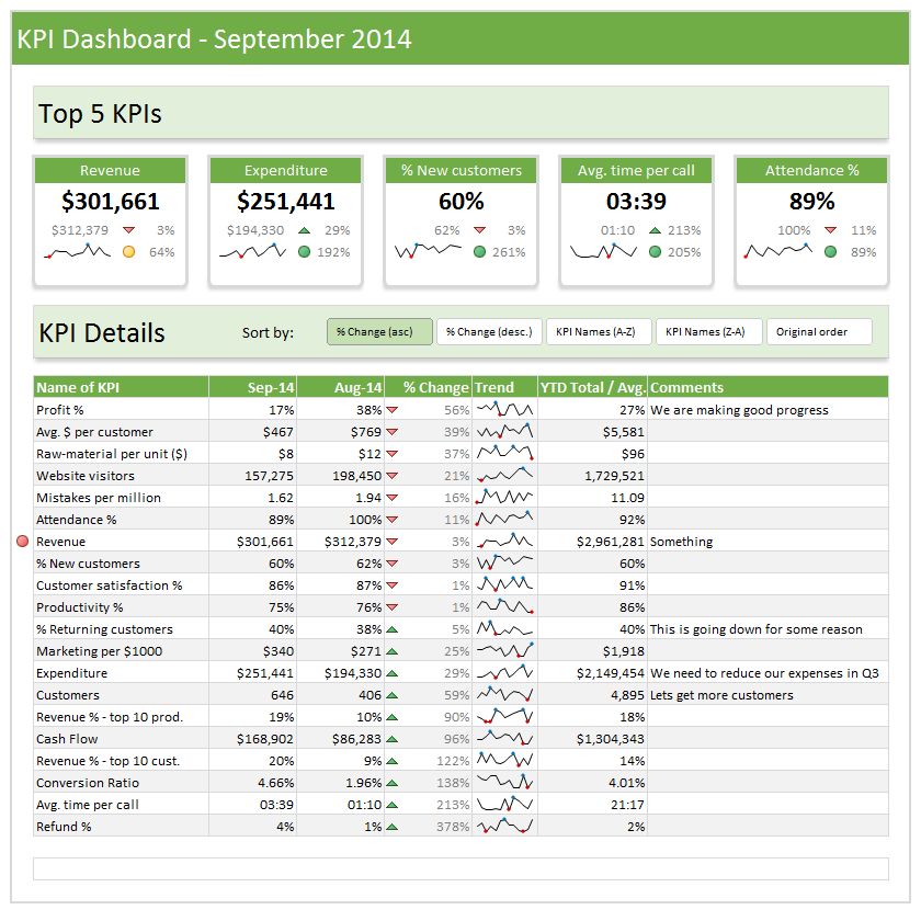
#2 – Introducing ready to use Dashboard Templates from Chandoo.org
This is the top most request from our customers & readers. A ready to use dashboard template that is easy, intuitive & awesome. So during the cyclone inflicted downtime, I created a set of ready to use dashboard templates. I am still polishing the product. This will launched on 13th of November (Thursday).
This is how our templates can help you:
- Type your data and generate beautiful dashboards. That simple.
- Generate 9 different dashboards from one set of data. Click & choose what you want.
- Customize with ease. Change currency codes, financial year starts etc.
- Build your own calculations and the template displays them just as beautifully.
- Ready to show, ready to print, ready to publish – All in one awesome bundle.
- Save time & worry about things that matter.
Here is a sneak-peek (click on it to enlarge):
#3 – 50 Ways to Analyze Data – Coming in Jan 2015
Last month I asked you to tell me the challenges you face when analyzing data. Based on all your feedback, I am designing an analytics course to help you most. It is 15% done. I will be completing rest of the course development during November & December.
![]()
So the 50 ways to analyze your data course will be launched on 21st of January 2015 (Wednesday).
Click here to sign up for the waiting list of this course.
I will email you details about the course as they get ready.
So that is all for now. Tomorrow, I will come back with an awesome Excel tip. Until then…


84 Responses to “Beam Me Up Scotty – Excel Hyperlinks”
I've just started using the formula version "=HYPERLINK("S:\Reserving\Management Judgment comments\check for MJ comments TOS 006 "&TEXT(month,"mmmm yyy")&".xls","MJ Comments")" and making it dynamic as some of the files that I use have a new name each month, or even each day.
I have an Excel file called "Important Stuff'. Rather than use post it notes, I put information I need into this file. I create hyperlinks to the files I most reference; especially when I have many different versions. I then add comments in the cells next to the hyperlinks to tell me what the differences are. I rarely have to search as everything is right there in the one file.
Great article! I'm bookmarking this for reference. Thanks for putting 'all you need to know about hyperlinks' in one place.
Hyperlinks are great but "Hyperlinks for navigating a spreadsheet are lost if saved as a "pdf". Even if you are utilizing Adobe Writer 8.0.0"
Great info! I never thought of using hyperlinks in Excel. Mostly used them in Word, email and especially in Powerpoint.
One cool thing I do is combine the hpyerlink function with a custom function I had help in building. I have a list of contractors from our Accounting Software (Quickbooks). We keep scanned copies of the 1099s in one folder. We can then download the data, which includes the vendors TaxPayer ID. The formula then checks for the file. If it exists, it provides a link to open it. If it doesn't it says so.
Here is the custom function code:
>>>>>>>>>>>>>>>>>>>>>>>>>
Public Function MyFileExists(MyFilePath As String) As Boolean
Dim objFSO As Object
Set objFSO = CreateObject("Scripting.FileSystemObject")
MyFileExists = objFSO.FileExists(MyFilePath)
Set objFSO = Nothing
End Function
>>>>>>>>>>>>>>>>>>>>>>>>>>>>>>>>>>>>>>>>
Bobby
BobbyBluford.com
This is aewsome. I have been using hyperlink since a long time. I like this option as this helps me create my Dashboard like a webpage. Thanks for sharing this, I got more insight of this option. 🙂
Bobby: Fantastic idea! What's amazing is as soon as I started reading 'scanned copies' in your post I was thinking 'hey that would be cool if you could just link to the files if and only if they exist'. Then you described how you do exactly that!
Nice one.
I use hyperlinks to jump from one location in a tab to another. When I add rows, the hyperlink destination location does not reflect the rows I just inserted. Does anyone know a way around this?
@All
If you like playing pranks on you co-workers or friends here is a simple Excel Hyperlink prank.
.
Open a workbook, probably not an overly important one, and select a page then either Use Ctrl A twice or select all the cells by clicking in the area to the upper left of A1.
Right click any cell and insert a Hyperlink, doesn't matter what its to, Another page, a Web Site or Send an Email
close the file
.
When anybody opens the file and clicks anywhere on the page it will execute the Hyperlink, even on a blank cell, where the Hyperlink isn't shown
This works particularly well on Blank worksheets
.
To remove right click anywhere on the page and Remove Hyperlinks
I have been wrestling hyperlinks to PDF files for over a year now, I can insert hyperlinks fine, and they look beautiful, but when click on them it comes up with "Cannot Open the Specified File". Does anyone know if this is because PDFs are unsupported by Excel or can other people get hyperlinks to PDFs working OK.
My application is a register of approved capital expenditure projects and the link is to a PDF scan of the signed approved document.
Did you add ".pdf" when you created the link?
I know this is an old comment, but we had the same problem too and the solution takes a little digging.
1. Open Adobe Reader X
2. Pick "Preferences" from the "Edit" menu
3. Pick the "General" category on the left.
4. Uncheck the "Enable Protected Mode at startup" box at the bottom.
5. Close Adobe Reader and retry opening the PDF file from Excel and it should work now.
Abobe Reader XI has a similar problem with a different error message. The settings in Reader XI seem to be Edit > Preferences > Security (Enhanced). At first I tried unchecking "Enable Protected Mode at startup" as this was the fix in Acrobat X. This did not work for me the first time. Then I tried unchecking "Enable Enhanced Security" and it started working. Then to test it, I re-checked both boxes... and it still works. I am not sure if other settings changed along the way, so I can't confirm the resolution other than "try this and see if it works!"
@JJ
What version of Excel are you using ?
and
What PDF Reader are you using ?
I assume you are using the Link to an Existing File or Web Page dialog?
Because that has worked as described for years without error
I am using excel 2007
The PDF reader I am using is Adobe Reader X.
So nothing really unusual.
I am using the Insert Ribbon, then the Hyperlink Icon.
I just had anohter play with it - it seems to work OK if the PDF file is on my C drive, but as soon as the PDF file is on a network drive it comes up with the error.
[...] Introduction to Excel Hyperlinks [...]
Dear Bobby i think your solution is very near to my requriment but can please explain in layman terms . I have a set of files in a folder let say a,b,c,d,e and i have a range of column in excel a1,b1,c1,d1,e1 .So if i click cell a1 file "a" should open. For range of 5 cells we can hyperlink each cell but if i have 100s of cells and files How can i apply hyperlink to all of them at once please explain
I'm using excel 2010 & adobe reader 10 - getting the same error "Cannot Open the Specified File” when linking to a file on a networked drive. File opens fine if it's on my PC.
Hope this helps.
Say in cell Z1, I have the URL: http://www.microsoft.com
And, I have a rectangle shape near A1... and I want it to have a hyperlink... and the URL for the hyperlink should be the URL in cell Z1.
So, when someone clicking the Rect will be taken to http://www.microsoft.com
When the URL is changed in cell Z1 to say http://www.yahoo.com
Now, when clicking the Rect should take him to the new URL.
How to achieve this? Thanks.
I am using Excel 2007. I have a spreadsheet with hyperlinks that were created using formulas, such as =HYPERLINK( Link Location, Name).
The hyperlinks work fine while I am in Excel, so I know they are active. However, when I use Acrobat 10 Pro to pdf the spreadsheet (and select the option to "Add Links") the Web links are no longer active.
I imagine it's because Acrobat cannot handle the "behind the scenes" commands such as a formula, and then just uses the visible text in that particular cell.
Has anyone found a work-a-round for this problem?
The problem is that the hyperlinks in Excel are nothing more than cell references. However the cell disappear when saving as .pdf.
In Powerpoint, the slide references can convert to pdf and continue to work.
[...] Hyperlinks: for accessing other parts of the workbook & data [...]
I have a single page dashboard created, where I would like each of the graphs to serve as a hyperlink to the actual data that creates the graph. The problem I'm running into is the URL for the hyperlink can be very long, depending on the data used to create the graph. Does anyone know how to get around the 255 characters limit Excel has on URLs? I used =Hyperlink(A1)&Hyperlink(A2) without Excel returning an error, but when I click on the link, it doesn't do anything. Any help would be greatly appreciated.
Brad,
I realize this comment is about 4 1/2 years old and you probably won't see this. But for anyone else who reads this, what about a URL shortening service like bitly, tinyurl, etc.?
I need to use hyperlink in excel to brows a web page according to each row
of a table that it's data comes from a external source such a sql connection.
but the text I have genarated from sql query "=hyperlink("Http://somthing.com","WebPage")"
appearing just like above text if i edit i in sheet for example adding some space after of before text and accepting changes then link become a real link
any kelp!
I would be appreciate
The simplest way to add web page links is:
1. In your browser, copy the url
2. Paste the url into a cell
3. Press F2
Done!
Hi Gents
i don't have not much knowledge about hyper link.Could please any
one can explain how hyper link has been working.
@Mohanraj
A hyperlink is like a shortcut
By selecti8ng the hyper link it takes you somewhere else
Hyperlinks can:
Take you some place else, like another sheet or workbook or open other file, they don't even have to be an Excel file
Hyperlinks can be placed in cells, ranges or objects in Worksheets like Charts or Rectangles etc, all of which trigger the hyper link when you click them
The post should tell you the rest of the story on how to use them
Hi I am trying to insert an activex control from Developer tab and add hyperlink (web address) to it. Hyperlink button is not enabled in Excel 2010. The same option is available in Excel 2007. I am trying to this by C# code using this function.
ActiveSheet.Hyperlinks.Add(ActiveXObject,"http:\\www.gmail.com",Type.Missing,"Screen Tip",Type.Missing);
This code throws 'invalid argument' exception. I tried to use 'Application.Selection' for anchor as first argument with out any success.
Any help is appreciated.
Regards,
Thanks with regard to providing these types of
good information.
Please tell any body..
Can we add a shortcut key as address of a hyperlink in Excel so that when we click on that hyper link the shortcut key works.
[…] Introduction to hyperlinks […]
I have an excel sheet with quite a lot of hyperlinks to files and folders in the server. We will be implementing new servers as part of a project, which means the directory structure of the old server will be moved to the new one.
Is there an easy way to keep the existing hyperlinks intact when moving to the new server? or do I have to edit each hyperlink and start all over again?
Your help on this much appreciated.
Cheers
ST
useful information
trying to hyperlink a cell with an object placed in shared folder.
It only kinks the shared folder but not the object in it...help!!!
I love the details on your websites. Thanks for your time!
Pl show me how to add a hypelink inside a text box, shape & image
so when I click any of the above it directs to hyperlink destination
Thanks
kanil
@Kanil
Simply insert a shape
Right click on the shape and select Hyperlink
I am trying to insert a .pdf file into an Excel spreadsheet. I have a large library of .pdf part drawings located on our server.
Path = Z:\MachineShop\Administration\Customer Drawings\
I would like the hyperlink to use a concatenated cell (C19) which contains =CONCATENATE(QUOTE!C1, QUOTE!D19)) QUOTE!C1 is the name of the file minus the .pdf suffix and QUOTE!D19 contains the .pdf suffix which is added to the part number to complete the file name. I would like the hyperlinked image to automatically load when a new value (part number) is entered into QUOTE!C1. Is this possible?
Trying to display only text if a parameter is/isn't found on a positive or negative IF response when using the IF and HYPERLINK functions together. If looking for a "No" value (positive) or if looking for a "Yes" value (negative); both are written correctly, to include the VBA macro, and what should drive a text-only response supplies a hyperlink that shouldn't be a hyperlink. It goes like this:
With Table1:
Positive No response:
=IF($O2="No", "Missing", IF($O2="Yes", HYPERLINK(pathname(), "Open"), HYPERLINK(alternatepathname(), "Open")))
Negative No response:
=IF($O2="Yes", HYPERLINK(pathname(), "Open"), IF($O2="Yes", HYPERLINK(alternatepathname(), "Open"), "Missing"))
Well, based on both responses, if Missing is displayed, it is a hyperlink, that points to nothing, instead of text. It looks like a flaw in Excel's coding. Is there a way to force just text to display?
As soon as I posted this, I found the answer.
The desired text-only response should still be writted with a HYPERLINK since one HYPERLINK function makes the entire cell followable regardless of the answer. In my case, I should write my formula like so:
=IF($O2=”No”, HYPERLINK("", "Missing", IF($O2="Yes", HYPERLINK(pathname(), "Open"), HYPERLINK(alternatepathname(), "Open")))
Having applied this, the hyperlink "look" still exists, but you can format over the cells. You don't have an active hyperlink, but you would still get the "pointer hand" like it were a hyperlink.
Hi,
I have an issue with Excel 2013. I am trying to add Navigation buttons to move around my workbook and I can't. I link the hyperlink to the place I want and try clicking the newly placed button/hyperlink and it throws up this Error Box message: ''Your organisation's policies are preventing us from completing this action for you. For more information please contact helpdesk.
Any ideas of what to check or change in Excel to be able to use hyperlinks? It was working a few days ago and now this nonsense!!
Thanks.
Without having Excel in front of me, you may want to check a few things.
File permissions in the folder your document is saved.
Make sure it isn't read-only.
If it is opened as an attachment, save it to your desktop first.
If it is saved to a network folder, try saving to your desktop.
See if you can add a trusted location for the document in Excel.
If you are still prohibited from this functionality, your group policy setting applied to your machine are probably restricting this action. You may have to look into whether you really need this functionality.
Hi All,
I have a question:
Is it possible to set hyperlink to an object?
What I mean is to follow the link to an object, not to put on an object.
For example, I have 10 pictures on my worksheets, I would like to set 10 hyperlinks on 10 cells (namely Pic 1, Pic 2, etc.) that will lead me to the corresponding pictures.
Is that possible?
Thanks in advance for your advice.
Cheers, 🙂
@MF
Yes,
Right click on the item, which can be a chart, shape, cell and Add/Insert Hyperlink
Set the location as a Range, Web address, external file etc
Hi Hui,
Thanks for your quick response.
However I want the link to be put on cell that will lead me to the object; not the other way.
Is it possible?
Why not put the pictures in a cell and link to the cell the picture is in?
Because the position of the object will be moved from time to time; and the picture is too big to be put into a single cell... 🙂
I link to charts often, and just merge cells or link to the upper left corner.
If it moves, that is trouble. Your best bet may be to run a macro to select it:
Sub SelectPicture()
Sheets("MyTab").Shapes("Picture 1").Select
End Sub
Thanks Mike for your suggestion.
I will give it a try. 🙂
I couldn't get the hyperlink formula to work and then found on some forums to put "#" before the sheet name..
so =HYPERLINK("#SHEET1!A1","WHY IN THE WORLD DOES THIS WORK")
does anyone know what the "#" does and why it is necessary?
thanks
Hi,
I have one excel document with four worksheets. The first sheet has the hyperlinks to the other worksheets. The issue I have is when I click on the hyperlink, it takes me directly to the source I need, but i find it hard to locate where the hyperlink has taken me on the screen, due to many cells of information being on the screen. So I'm wondering is there anyway of highlighting the cell that the hyperlink takes me to (ie: the source) or highlighting the borders of the source once I jumped there.
Hi
I have a workbook that I have created and am using a hyperlink to navigate to another page however I would like the info from the previous page NOT to save is there a way to do this?
@Angela
You could probably do this using some VBA Code
I'd suggest posting the question on the Forums and attach a sample file
http://forum.chandoo.org/
Explain exactly what you want to achieve
I am trying to create a hyperlink or formula that will generate an email but also include the file I am in as an attachment.
@Chandan
I doubt that can all be done by a simple Hyperlink
It could be done with a small piece of VBA Code
I'd suggest using the search box at the top right of this page as I am pretty sure that has been answered before
Thank you for the excellent tutorial. Pls help me on how to create a link in excel to open a specific page in pdf. I have use several code to do this but still take me to page of the pdf file. How do I do this to jump to a specific page directly by clicking a link from excel. Thank
@Muffliu
Try:
=hyperlink("E:\testfile.pdf#page=5")
I have an excel document with hyperlinks to a folder on my desktop. I now want to share the document, but am struggling to keep the hyperlinks working. When others open the file, I get an error that the internet site reports that the item requested cannot be found. Is there a work around that doesn't require re-hyperlinking all of the documents?
Hello,
Well we use a particular software for document management made by humming bird software. This software is supposed to be a last version Archive save. That is not what it is used for at our work though it is used as an active directory. I was wondering if anyone has recent experience with hyperlinking between two or more documents in this type of storage.
Is there a hyperlinks for dummies? I need to link a pdf in an excel spreadsheet from my PC. I want to be able to email it to send it by email and be able to open spread sheet with the link on smart phone. Please help!
Repeat the process of coloring and ironing until you like what
you see.
I have two mysteries in Excel 2010:
1. I was given a spreadsheet in which numerous cells were formatted with hyperlinks and asked to extract the hyperlinks so they could be viewed directly in adjacent cells. I never found a function that could do that and didn't have months to take a class to learn to use VBA.
2. When you type a URL into a cell and hit enter, Excel converts the formatting of that cell so that it becomes hyperlinked. I have a spreadsheet that stopped doing that. In fact, the Insert Hyperlink command has been disabled in the ribbon and in the right-click menu. (However, the =hyperlink("") function still works.) How did that happen, and how do I get the command back?
I checked File > Options > Proofing. Nothing was out of the ordinary there.
@Rich
Can you please ask the question in the Chandoo.org Forum http://forum.chandoo.org/
There are a number of ways Hyperlinks can be added and so attaching a sample file would be great and will speed up an answer
Appreciating the dedication you put into your site and detailed information you present.
It's awesome to come across a blog every once in a while
that isn't the same out of date rehashed information. Wonderful read!
I've bookmarked your site and I'm adding your RSS feeds to my Google account.
How can you make the entire cell active? Normally only the text within the cell becomes active and the remaining white space only selects the cell. Example: if the cell columnwidth is say 30 but the hyperlink textToDisplay is "XYZ" then only "XYZ" will be the active portion and all the empty space within the cell is not.
There is an exception. If the cell is formatted with an indention then the entire cell becomes active. For my purpose this exception can be used but I desire to have the cell text centered. But sometimes the cell width is just a fraction larger than the width of the text so indention would break the desired formatting. This is why I would like to have the entire cell hyperlink active and the textToDisplay centered without an indent.
When I originally commented I seem to have clicked the -Notify me when new comments are added- checkbox and now whenever a comment is added
I receive four emails with the exact same comment.
Perhaps there is a way you are able to remove me from that service?
Thank you!
Fantastic beat ! I wish to apprentice at the same time
as you amend your web site, how can i subscribe for a
blog web site? The account helped me a applicable deal. I have been a little bit acquainted of this your broadcast provided bright
transparent idea
Heya superb blog! Does running a blog such as this take a massive amount work?
I have very little understanding of programming but I was hoping to start my own blog in the near future.
Anyway, if you have any recommendations or tips for
new blog owners please share. I know this is off subject however I just needed to
ask. Kudos!
Thanks to my father who shared with me on the topic of this blog, this
blog is really remarkable.
Hello, I would like to subscribe for this web
site to take latest updates, thus where can i do it please help out.
Awesome blog you have here but I was curious about if you knew of any discussion boards that cover the same topics discussed in this article?
I'd really like to be a part of online community where I can get comments from other knowledgeable people that share the same interest.
If you have any suggestions, please let me know. Bless you!
@Promiennik
You may want to look at the Chandoo.org Forums, a very vibrant community for asking Excel questions
http://forum.chandoo.org/
With havin so much content and articles do you ever run into any issues of plagorism or copyright violation?
My blog has a lot of unique content I've either created myself or outsourced but it
appears a lot of it is popping it up all over the
web without my authorization. Do you know any methods
to help protect against content from being stolen? I'd really
appreciate it.
I am having difficulty in opening a hyperlink to a pdf that is housed on the internet (an internet hyperlink ending in .pdf). When I first click the link in excel, I get an alert which says: "Opening.....pdf. Some files can contain viruses or otherwise be harmful to your computer.... Would you like to open? I click OK, and then I get an Excel error that says "Unable to open https://......pdf. The internet site report that a connection was established but the data is not available. How do I get around this? I can copy the hyperlink out of Excel, paste it into my web browser and it opens without any problems. Thanks.
Great goods from you, man. I've be aware your stuff prior
to and you are just extremely great. I really like what you've received here, certainly like what you're saying and the
way in which through which you are saying it.
You make it enjoyable and you still care for to keep it wise.
I can not wait to read much more from you. That is actually a wonderful web
site.
I tried the FoloowHyperlink worksheet event for a hyperlink text in a cell; attached some code to it, and it worked well. When I created a second hyperlink and attached some other code to this hyperlink in another cell, and clicked it, it worked but the result was not what I expected. The second hyperlink executed the code meant for the first hyperlink.
The questions are:
1. Whether the FoloowHyperlink event works for only one hyperlink in one sheet?
2. If not, how many hyperlinks can I create in ONE sheet and attach different code to them. How?
I really appreciate your piece of work, Great post.
We're a bunch of volunteers and starting a new scheme in our community.
Your web site provided us with useful information to work on. You have performed
an impressive activity and our entire group will likely be grateful to you.
I have a Master Excel Workbook in which i have linked the relative documents using hyperlinks. These workbooks open when i click on the Hyperlink. i have also created a back Link to Direct back to the Master. But in the process when i get directed back to Master Excel Workbook the Other Workbook which opened by clicking hyperlink remains open. I want those opened workbooks to close when i click back to master file. Is there a way in which i go directly to the master Excel Workbook by simultaneously closing the other Workbook.
Appreciation to my father who told me concerning this web site,
this website is genuinely awesome.
It's a pity you don't have a donate button! I'd certainly
donate to this superb blog! I guess for now i'll settle for bookmarking and adding your RSS
feed to my Google account. I look forward to brand new updates and will talk about this site with my Facebook
group. Talk soon!
@Forex
You may want to visit this page:
https://chandoo.org/forum/threads/donate-support-our-ninjas.18150/
Awesome post.