

This week many Excel bloggers are celebrating VLOOKUP week. So I wanted to chip in and give you a comprehensive guide to VLOOKUP & Other lookup formulas. Read on …,
What is VLOOKUP Formula & how to use it?
I tell my excel school students that learning VLOOKUP formulas will change your basic approach towards data. You will suddenly feel that you have discovered a superman cape in your attic. It is that awesome.
What does VLOOKUP really do?
Imagine you have a list of data and you want answer a question like, “How many sales did Jimmy make?”
VLOOKUP is one of the formulas you can use in this situation. VLOOKUP searches a list for a value in left most column and returns corresponding value from adjacent columns.

Read more – What is VLOOKUP formula and how to use it?
Introduction to VLOOKUP, MATCH & OFFSET formulas
VLOOKUP may not make you tall, rich and famous, but learning it can certainly give you wings. It makes you to connect two different tabular lists and saves a ton of time. In my opinion understanding VLOOKUP, OFFSET and MATCH worksheet formulas can transform you from normal excel user to a data processing beast.

Read more – VLOOKUP, MATCH & OFFSET explained in plain English
How to do wildcard searches with VLOOKUP?
Often we need our lookup formulas to go wild. Not in the sense of go-wild-and-chomp-a-few-kilo-bytes-of-data sense. But wild like wild cards. For eg. In the below data, we may not remember the full name of sales person, but we know that her name starts with jac. Now how do you get the sales amount for that person?
You can use wildcard characters * and ? with VLOOKUP & several other Excel formulas.

Read more – Using wildcards with VLOOKUP formulas
Making VLOOKUPS dynamic with data validation
Sometimes we don’t know what we want. If this happens when I am in a bar, I usually order a cocktail. Just a mix of everything. The same will work in Excel too.
For eg. If you have lots of data, but the value you want to look up needs to change based on whims and fancies of your users, then you can resort to a cocktail. A mix of VLOOKUP with Drop down lists (Data validation).
Read more – Use data validation with VLOOKUP to lookup anything you want
How to lookup values to the left?
There is no argument that VLOOKUP is a beautiful & useful formula. But it suffers from one nagging limitation. It cannot go left.
Let me explain, Imagine you have data like below. Now, if you want to find-out who is the sales person who made $2,133 in sales, there is no way VLOOKUP can come to rescue. This is because, once you search a list using VLOOKUP, you can only return corresponding items from the column at right, not at left.
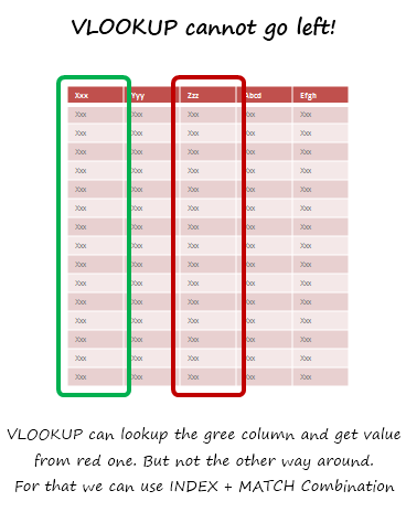
Read more – How to use INDEX + MATCH combination to fetch values from left
How to lookup based on multiple conditions?
Not always we want to lookup values based on one search parameter. For eg. Imagine you have data like below and you want to find how much sales Joseph made in January 2007 in North region for product “Fast car”? Read more to find how to solve this.
Read more – How to lookup based on multiple conditions?
How to get values from multiple columns with VLOOKUP?
VLOOKUP is great for extracting information from a huge data table based on what you are looking for. But what if you need to extract more than one column of information? For eg. Lets say you have salesperson’s name in left most column, and monthly sales figures in next columns, one for each month. Now, you want to find the total sales made by a given sales person. How do you go about it?
Read more – How to get values from multiple columns with VLOOKUP?
Using VLOOKUP formula with tables
Excel Tables, a newly introduced feature in Excel 2007 is a very powerful way to manage & work with tabular data. I really like tables feature and use them often. If you are new to tables, read up Introduction to Excel Tables. In this short video, understand how to use tables with VLOOKUP formulas.
Watch the video – Using VLOOKUP formula with tables
Doing 2 way lookups in Excel
So far we have seen what VLOOKUP formula is and how to put it to some nifty uses. Lets go one step further and learn how to do 2 Way Lookups.
What is a 2 Way Lookup?
Lookup is when you find a value in one column and get the corresponding element from other columns. 2 Way Lookup is when you lookup value at the interesection of a given row & column values.
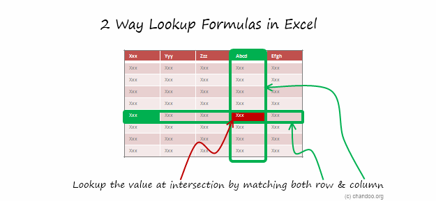
Read more – 2 way lookup formula in Excel
Getting 2nd matching value from a list using VLOOKUP
We know that VLOOKUP formula is useful to fetch the first matching item from a list. So what would you do if you need 2nd (or 3rd etc.) matching item from a list?
Read more – Getting 2nd matching value using VLOOKUP
Range lookups in Excel
Here is a really tricky problem. Recently I was given a data set like this (shown below) and asked to find the position of lookup value in the list. The only glitch is that, instead of values, the lookup table contained lower and upper boundaries of the values. See the below illustration to understand the situation. In this case, how do you lookup?
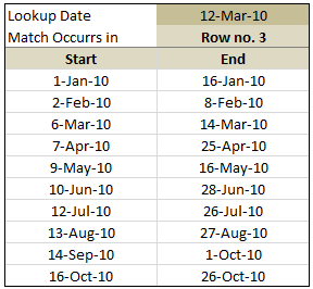
Read more – Doing range lookups in Excel
6 VLOOKUP tips
Ok, you have learned how to write vlookup formulas. You have also seen some pretty interesting examples of it.
But how do you write better VLOOKUP formulas?
Read more – 6 VLOOKUP tips
FREE VLOOKUP cheat sheet – Download today
Please download free VLOOKUP formula cheat-sheet. This cheat-sheet is prepared by Cheater John specifically for our readers. I hope you enjoy the one page help on VLOOKUP.
Download FREE VLOOKUP cheat sheet
Your Favorite VLOOKUP Tips?
When I am working with data, not a day goes by without using some sort of lookup function. I use VLOOKUP, MATCH, INDEX, OFFSET, SUMIFS, SUMPRODUCT, GETPIVOTDATA in most of my dashboards & reports. These are easy to use once you understand the syntax and technique.
What about you? What are your favorite tips on VLOOKUP? How do you use lookup formulas? Please share using comments.
Want to Learn More Formulas? Get my VLOOKUP book
If you want to learn VLOOKUP and other Excel lookup functions, then consider getting my VLOOKUP book.

|
Comprehensive and easy to understand
This is a book for everyone who uses Vlookup. Most of us think… Oh.. I already know the function. But this book will open your eyes to some brilliant techniques. – By Dr. Nitin Paranjape
Solid introduction to lookup functions
This books does a wonderful job of taking each of the lookup functions available in Excel, breaking them down to a simple, easy-to-understand level. – by Lucas Moraga |


14 Responses to “How to Add your Macros to QAT or Excel toolbars?”
We have only just got excel 2007 so this is helping me navigate my way through the differences cheers.
For Macro's i always add a Command Button, rename it something obvious, change the colour of it and finally add the following to its View Code section.
Application.Run "MAcro1"
This way anyone opening the file knows what to do if i ever win the lottery and dont make it in 🙂
Hi,
Good article. But I have this problem.
1) Customized QAT with a macro. Macro name = MacroX
2) Runs OK from original location (e.g. C:\TestLoaction1\TestFile.xls)
3) Copy past file to new location (e.g. C:\TestLoaction2\TestFile.xls)
Menu button now fails:
Cannot run the macro "C:\TestLoaction1\TestFile.xls'!MacroX' The macro may not be available in this workbook...
Of course the code is there, and macros are enabled.
Could get it to work after deleting and recreating macro custom buttons. So have to re-assign macro to QAT button every time I move the file?
If I put a form button on he worksheet and assign the macro to that, it's location independent.
Any ideas?
Thanks
@Ron
What you have said is correct
Macros within a worksheet are stored within the worksheet and hence follow it.
Macros referenced by a button in the QAT or elsewhere are locaed in a file and if that file is moved the linkages don't follow.
The easiest way around this is to store all your macros in a location that doesn't move and is in fact reloaded everytime that Excel starts and that is called the Personal.xlsx/b file.
These are refered to several time at Chandoo.org or have a read of
http://www.rondebruin.nl/personal.htm
or
http://office.microsoft.com/en-us/excel-help/deploy-your-excel-macros-from-a-central-file-HA001087296.aspx
In Excel 2003 and prior versions, a button added to the Toolbar maintained a DYNAMIC link to the file (e.g. Personal.xlsb) holding the assigned macro, such that if the file was relocated for any reason (by using Excel's native Save As command rather than just moving it via Windows Explorer), the link between the button and the file was updated.
I expected the same to occur with Excel 2007+, but alas, Microsoft in their infinite wisdom have removed another feature useful to advanced users (just as they did by removing the ability to design your own buttons)!!
So having just done some reorganisation of my files, I now have to remove and recreate every friggin macro button on my QAT (I have lots) - what a pain in the proverbial!!
Hi Hui,
Thanks for the help, that's really useful.
1) The macros I'm adding are for one specific Excel application, so I really wanted the macros to follow the file
2) I didn't want to have to pass other files around too and have users installing those - either Personal.xlsx/b or as an Add-In.
3) I realise now that the QAT additions will appear for other Excel workbooks in which I don't want the macros available.
So, it looks like I need to keep it local, by using a button on the worksheet. Unless you can suggest any way of adding to menus just for a specific workbook.
Thanks again for your help. Great site, so I'll be signing up for the emails.
Ron
I know I'm a little late jumping on this post, but wondering if anyone knows how to add a UDF to the QAT? I've saved my UDF in my personal workbook, but it does not show up in my list when I choose Macros when customizing my QAT. Suggestions? Thanks!!
@Cheryl: UDFs cannot be accessed like Macros. You can use them from other macros or from worksheet cells as formulas...
@David: If you save your macros file and then install it as an add-in then it will be always available for you.
The instructions work great when you are creating a new file, and it is still open. I find that I can't access macros after I've saved a file as an xlam and closed it. When I reopen the xlam, either by browsing to it, or by having it set to open as an addin using Excel Options, the macros are no longer available in the macros list when I go to edit the QAT. Any way around that?
[...] Add this macro as a button to Quick Access Toolbar [...]
I need to create a button that will run a macro. Once you click the button it needs to open up a browser asking you to select a report/file. Once you select the file, it will run the macro on the selected file and then save it as a new report with a name and the current date. I created the macro to sort/modify the report but I do not know how to do what I mentioned above. I hope this makes sense.
I'm having trouble adding a macro to the QAT. I've done everything up to step 5 but my macro isn't showing up. What am I doing wrong?
[...] Add Macros to Quick Access Toolbar (works in Excel 2003 & above) [...]
Hi,
Thank you for the explanation. Very useful for a recent switcher from office 2003 to office 2010.
My follow-up question is: in Excel (or ppt) 2010, can you customize the macro button that you put in the QAT?
In office 2003, once you chose the custom button for your Macro, you could then edit pixel by pixel the said button.
For instance, I've created 2 Macros in PPT that are converting all my slides to either English or French language, so I'd like one button to show EN and the other FR... that would be more meaningful that any of the possible "custom" office 2010 buttons
I read all the post and one important aspect to the QAT was never mentioned. That is, you have a macro driven worksheet that you want to share with other. You have customized the QAT with two icons to run the macros (VBA programs in reality). However, when the others receive the workbook, the icons are no where to be found. It's my understanding those "customized buttons" have been saved to an outside file, Excel.qat. QUESTION: Could one simply attach that file to your email, along with the worksheet, and tell the recipients to copy that file to correct location on their computer - C:\Users\\AppData\Local\Microsoft\Office|\
Would the customize macro buttons then appear in the worksheet and, more importantly, work? Thanks for your thoughtfulness and thanks for well written instructions Chandoo!
MortW