
Once in a while everyone is bound to come across this problem. You type a formula in a cell, then you press ENTER. Bam! nothing happens. You check if a donut chunk went in to the key board and some how jammed the ENTER key. So press it again, this time harder. But nothing. Excel formula showing as text instead of actual result, like this:
Now what to do?
Of course, you can be careful when eating donuts. But careful donuts sure sounds like a paradox. So instead lets roll up our sleeves and find out the reason for this mishap.
The top reason for Excel formula showing as text :
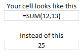
You may have accidentally pressed CTRL+` (back quote symbol, the key below escape key in your keyboard) or activated the “Show Formulas” mode in Excel. 
When you do it, excel shows the formulas instead of their results.
To fix this error and get back the values (or results) just press CTRL+` again or click on the “Show formulas button”
The next reason why formulas are shown as formulas:
You may have set the cell formatting to “Text” and then typed the formula in it.

When you set the cell formatting to “Text”, Excel treats the formula as text and shows it instead of evaluating it.
To fix this error, just select the cell, set its formatting to “General”. Now edit the formula and press enter. (Alternatively you can press F2 and then Enter after setting format to General).
The less probable reason why formulas are shown as formulas instead of values:
You may have accidentally typed a single quote ‘ before the = sign in the formula.

When you type single quote ‘ in a cell excel treats the cell contents as text and does not evaluate any formulas within.
To fix this error, just remove the single quote.
What is your experience with excel formula errors?
The very first time I pressed CTRL+` by accident, it nearly freaked me out. All the columns became too wide and the formatting went for a toss. Everything looked weird. It took me a while to figure out that I accidentally pressed the Show Formulas shortcut (CTRL+`). I felt huge relief when I got the results back.
What about you? Did the formula error ever freaked you out? What other things about formulas worry you? Pls. share using comments.


12 Responses to “29 Excel Formula Tips for all Occasions [and proof that PHD readers truly rock]”
Some great contributions here.
Gotta love the Friday 13th formula 😀
Great tips from you all! Thanks a lot for sharing! bsamson, particularly you helped me on a terribly annoying task. 🙂
(BTW, Chandoo, it's not exactly "Find if a range is normally distributed" what my suggestion does. It checks if two proportions are statistically different. I probably gave you a bad explanation on twitter, but it'd be probably better if you fix it here... 🙂 )
Great compilation Chandoo
For the "Clean your text before you lookup"
=VLOOKUP(CLEAN(TRIM(E20)),F5:G18,2,0)
I would like to share a method to convert a number-stored-as-text before you lookup:
=VLOOKUP(E20+0,F5:G18,2,0)
@Peder, yeah, I loved that formula
@Aires: Sorry, I misunderstood your formula. Corrected the heading now.
@John.. that is a cool tip.
Hey Chandoo,
That p-value formula is really great for a statistics person like me.
What a p-value essentially is, is the probability that the results obtained from a statistical test aren't valid. So for example, if my p value is .05, there's a 5% probability that my results are wrong.
You can play with this if you install the Data Analysis Toolpak (which will perform some statistical tests for you AND provide the P Value.)
Let's say for example I've got two weeks of data (separated into columns) with the number of hours worked per day. I want to find out if the total number of hours I worked in week two were really all the different than week one.
Week1 Week2
10 11
12 9
9 10
7 8
5 8
Go to Data > Data Analysis > T-Test Assuming Unequal Variances > OK
In the Variable 1 Box, select the range of data for week 1.
In the Variable 2 Box, select the range of data for week 2.
Check "Labels"
In the Alpha box, select a value (in percentage terms) for how tolerant you are of error.
.05 is the general standard; that is to say I am willing to accept a 95% level of confidence that my result is accuarate.
Select a range output.
Excel calculates a number of results: Average (mean) for each week's data, etc.
You'll notice however that there are two P Values; one-tail and two-tail. (one tail tests are for > or .05), the number of hours I worked in week two is statistically equivalent to the number of hours I worked in week one.
So here’s a way you might want to use this. You put up a new entry on your blog. You think it’s the best entry ever! So you pull your webstats for this week and compare it to last week. You gather data for each week on the length of time a visitor spends on your website. The question you’re trying to prove statistically is whether there’s an average increase in the amount of time spent on your website this week as compared to last week (as a result of your fancy new blog post). You can run the same statistical test I illustrated above to find out. Incidentally, it matters very little to the stat test whether the quantity of visitors differs or not.
Anyhow, the Data Analysis toolpack doesn't perform a lot of stat tests that folks like me would like to have access to. In those cases I have to either use different software, or write some very complicated mathematical formulas. Having this p-value formula makes my life a LOT easier!
Thanks!
Eric~
Fantastic stuf..One line explanation is cool.
Thanks to all the contributors
OS
Take FirstName, MI, LastName in access (you can fix it to work in excel) capitalize first letter of each and lowercase the rest and add ". " if MI exists then same for last name:
Full Name: Format(Left([FirstName],1),">") & Format(Right([FirstName]),Len([FirstName])-1),"") & ". ","") & Format(Left([LastName],1),">") & Format(Right([LastName],Len([LastName])-1),"<")
I teach excel, access, etc etc for a living and i have my access students build this formula one step at a time from the inside out to show how formulas can be made even if it looks complicated. Yes I know I could just do IsNull([MI]) and reverse the order in the Iif() function but the point here is to nest as many functions as possible one by one (also I illustrate how it will fail without the Not() as it is)
Extract the month from a date
The easiest formula for this is =MONTH(a1)
It will return a 1 for January, 2 for February etc.
if in a column we write the value of total person for eg. 10 if we spent 1.33 paise each person then how we get total amount in next column and the result will in round form plzzzzz solve my problem sir................... thank u
@Anjali
If the value 10 is in B2 and 1.33 paise is in C2 the formula in D2 could be =B2*C2
If the values are a column of values you can copy the formula down by copy/paste or drag the small black handle at the bottom right corner of cell D2
kindly share with me new forumulas.
How to convert a figure like 870.70 into 870 but 871.70 into 880 using excel formula ? Please help.