
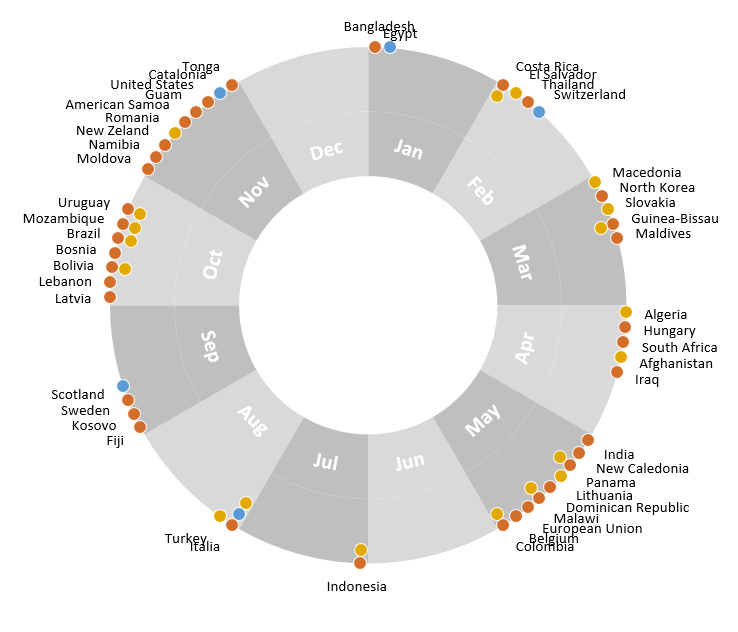
Few days ago, we learned how to create a pie+donut combination chart to visualize polls around the world in 2014. It generated quite a bit of interesting discussion (47 comments so far). One of the comments was from Roberto, who along with Kris & Gábor runs The FrankensTeam an online library of advanced Excel tricks, charts and other mind-boggling spreadsheet wizardry.
I really liked Roberto’s comments on the original post and a charting solution he presented. So I asked him if he can do a guest post explaining the technique to our audience. He obliged and here we go.
Over to FrankensTeam.
Combine pie and xy scatter charts – guest post by The FrankensTeam
Fraü Blucher: I am Fraü Blucher. [horses whinny]
Igor: Steady.
Freddy: Uh, how do you do? I am Dr. Fronkensteen. This is my assistant. Inga, may I present Fraü Blucher. [horses whinny] I wonder what’s got into them.
First of all, we would like to say thank you to Chandoo for asking us to explain how to make this kind of chart.
Recently we have seen an interesting pie-based plot chart by Chandoo. Our proposed version combines 3 different chart types based on some background calculations. The final model is dynamic, you can add more data, and you have the choice to use 1D or 2D data table. All the calculations are prepared on the sheets up to 10 categories. In this guest post we would like to share our template file and show you some of our charting technique.
As an extra, at the end of the post you can find a link to our VBA code which could be used to rotate the chart labels.
Building blocks of the vote-chart
We combined 3 chart types:
- donut chart (two series)
- Outer grey slices
- Inner grey slices with month names
- pie chart (one series)
- Invisible data for placing country labels
- xy scatter chart (three series)
- Brown dots – Legislative
- Blue dots – President
- Orange dots – Referendum
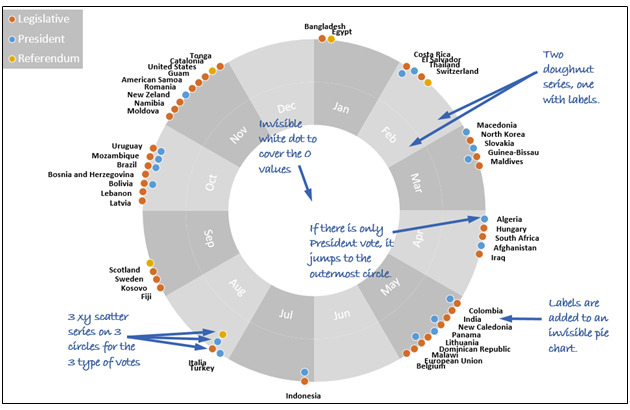
Doughnut series
The two series: month_label and month serve to create the gray ring for the months.
The labels in a doughnut chart are always positioned at the center. By using two series (so two rings) and eliminating the border lines, the two rings seem to be one, but the labels can be positioned at the bottom by adding it to the innermost ring. The reason why we use two rings instead of moving the labels manually is very simple: this way the labels will always stay at the same position, even if you resize the chart. Also it is easier than manually adjust the label boxes.
The month names are linked to the labels from cells (you can see it on the formula bar if you click on one label) because only one axis label could be assigned to the chart, and we use it for the country names (those are more… :-))
XY scatter series
Scatter series are used to arrange the colored dots on the outer ring. This is a main difference from Chandoo’s version. We use 3 series to separate the three different vote categories: presidential, legislative and referendum, and to position the dots of the same country in radial direction as you can see on the original chart. The 3 series form 3 big circles with different radius: legislative is the outermost, referendum is the innermost, but we move the points from the inner circles to the outer, if there is no “higher” vote-type.
Naturally it is possible to adjust the size and shape of the indicators.
We will show you later how to calculate the scatter point positions. (Maybe at first sight it seems to be difficult but you will see it is easy to arrange them properly.)
Our file is prepared to handle more vote-types (or other categories). You will only need to add the new series to the chart!
Pie series
Pie chart is used to position and show labels with the names of the states. The chart itself is hidden (we set to no color and no line) so only the labels are visible.
The number of slices of the pie is determined by the maximum number of countries per month – it needs to be multiplied by 12. All the slices are sized equally and all has a label, but only the ones that we need will have the name of the state, for the rest, the label is an empty string “”.
Formulas behind the chart
For better understanding we separated the data and the support formulas to two sheets. We prepared the file to be able to work with two different types of data table.
You may have the type of vote in one column (1D):

Using some formulas, this table could easily be re-ordered to a pivot-table-like 2D format. This is what you can see in our file on sheet Transpose_data:

This table is the starting point to build up the help data for the charts.
You can find all the calculations on Support sheet. A key element of calculations is the total number of slices for the pie chart. We need to determine the maximum number of countries per month – this will be the number of slices for each month. We use a named formula: max_size_month for this data (here we adapted Chandoo’s MODE-based formula).
The total number of slices will be 12*max_size_month.
The second step is to determine the slice number for each country, and based on that, calculate the the slice angle in radians. If you think about trigonometry, you will remember that sine and cosine together with radius determines the x and y coordinates of the circle points.
We created a calculation table with the necessary formulas. This table is dynamic and prepared to process more data rows and more vote (or other) categories.

The dots are positioned on 3 circles. We use a fixed parameter in a name: circle_distance to set the radiuses of the circles.
We use a support range for both text labels: country names and month. For month names we avoid to use TEXT function with string parameter “mmm” because in non-english systems it will not work! Instead we use Custom cell formatting with code “mmm” – this kind of formatting is translated automatically to locals.
For country names we set the country to the same pie-slice where the dots are, all the rest will have an empty string as label. The column with country name formula will be assigned to the category axis of the chart, but the month names will be linked to the doughnut-series labels one by one, because it is not possible to set two different axis labels. 🙁
How to put it together?
- Select the Legislative x and Legislative y columns, and create a scatter chart.
- Add two more series using the President x and y and Referendum x and y columns.
- Set the axis minimum to -1 maximum to +1 for both of the axes.
- Delete the axes and the grid lines. You can see something like this:

The dots do not form a circle yet, but after you add the pie chart, the shape of the plot area will be a perfect square, so the circle will appear. - Add a new series named for_label using arr_pie both for x and y values:

- Set the chart type of this series to pie and set no fill, no border. Now the dots form perfect circle.
- Link the category axis for this data series to the support column with Label States. (In the Select Data dialogue box click on the “for_label” series, then the Edit button. Select the range from the sheet.)
- Add labels to the pie slices. Set it to show Category name and position Outside end.
- Add two more series (month and month_label) using arr_12 for the values.
- Set the chart type of these two series to doughnut, and set no borders. Color every second slice to darker gray.
- Add data labels for the inner circle, and link the labels one by one to the sheet cells with month names. (Select one label, click on the formula bar, type = and click on the appropriate cell you want to link the label to.)
- Finally you have to hide the 0 data points which appear in the middle of the chart. Add a new xy data series (named “white series”) with fixed values ={0} for x and y. Set a marker of series to the same color as the background of your chart, and use a marker large enough to cover the unnecessary point. 🙂
+1. You can add new xy series if you need – the calculations are already done on the sheets. It is not problem to use over-sized ranges, the error values will become 0 and will appear in the center of the circle – covered by the white series. BUT important for the proper covering, the white series must be the very-last series, so after adding new series, check the order, and move the white series to the bottom of the list.
Bonus: rotate the chart labels using VBA
As you can see on the above picture all the labels are horizontal. To rotate it to radial direction a piece of VBA code is needed. We created this code and published on our site – please feel free to use it for this chart or your other charts (see the link below).

Download the example files
Click here to download the files. Examine the formulas, chart settings and formatting to learn more. This is a highly advanced chart, so take some time to go thru it. You will learn a lot.
Learning points and links:
- Be careful using TEXT formula with string parameter in international environment! You can read about it here.
- Combining xy scatter with pie chart makes the plot area shape perfect square, so it is easy to create a perfect square area for drawing by the xy coordinates. You can read about it here.
- Rotate chart labels to radial or tangential direction is possible with this VBA code.
Added by Chandoo:
Thank you Frankens Team
Thank you so much Robert, Kris and Gábor for taking time to write this. It is a pleasure hosting your article here. I have been following your website for several months and every time I visit it, I end up learning something interesting, creative and just plain awesome. Thanks for sharing your knowledge, ideas and technique with all of us.
Like this chart? Say thanks to Frankens Team
If you enjoyed this chart, please say thanks to Frankens Team. Also visit their site to see how far you can with Excel.


11 Responses
Thanks for an excellent Year plan chart.
//Ola
I quickly took the 1D version, moved all calculations to the Input sheet (to make it slimmer) – had to replace some =COLUMN() with COLUMNS() and =ROW() with ROWS(). It works fine except it still throws ‘A formula…invalid references’ error. … to be found.
If I was running a business and needed this kind of business information to make a strategic decision on, and if I paid people by the hour, then I would not want my people to produce this nice looking chart.
Why? Because it takes much longer to produce this nice looking chart than a simple boring-looking table, and that extra time adds no benefit to my strategic decision as far as I can see. My people could have been doing something more valuable with their time.
If I was selling a magazine, then I’d consider it a valid choice to do the complete opposite if I thought it would help my product to stand out in the minds of consumers. Because the magazine’s primary purpose is to sell.
I think that the time spent (little or much) in a job done badly is always time misspent and as you said “My people could have been doing something more valuable with their time”
on the contrary, if I have a job well done my money was well spent … may have spent too much … but at least I’ll be satisfied with the result.
Having said that, I really enjoyed your recent chart so I’d like to see how you would have done this work too.
P.S.
maybe your answer to my question came here by mistake?
Great chart, thanks for the step-by-step.
I’ve tried recreating this, but slightly different; I’ve used it as a calendar, splitting the ‘slices’ into 3 days chunks and then placing my items into the slices, catagoriesed as different item types (eg Birthday, holiday etc instead of legislative, president etc.). Then the idea was to have the labels start with the date (eg. 22. National Day).
However, the last part I can’t get to work is getting the labels onto the ‘for_label’ pie. I’ve linked to the category data set, set the labels up on the chart but: (a) they dont show my text labels, they are all just a ‘1’ and (b) they are not spacing out around the pie chart to line up with the scatter dots, they are along the first 15 pie slices (even though my labels data has the labels spread out along the 120 slices with “” between them).
Any thoughts? Thanks in advance.
@Neil
Maybe you can send the file to my e-mail (robb.men from gmail.com)? Before you send, please remember to delete sensitive data
Roberto – thanks. Was just opening to check before sending and I noticed that it had ‘fixed’ itself upon opening. When I moved the chart to a new location, it again didn’t work putting 1’s in all the labels, but opening and closing the workbook seems to make it refresh. Not perfect, but not something to worry about. Thanks anyway.
@Neil
very well 🙂
I really like the version with labels rotated to radial direction… look at the chapter: “Bonus: rotate the chart labels using VBA” and if you need help please contact us
I am unable to format doughnut series to display months on them. Legend is appearing outside the chart
I can’t load the VBA-version :O – empty version …
… Chandoo – please help 🙂
Thx Stef@n