How to use Excel Data Model & Relationships

Share

Facebook
Twitter
LinkedIn

Have you ever been in a VLOOKUP hell?

Its what happens when you have to write a lot of vlookup formulas before you can start analyzing your data. Every day, millions of analysts and managers enter VLOOKUP hell and suffer. They connect table 1 with table 2 so that all the data needed for making that pivot report is on one place. If you are one of those, then you are going to love Excel’s data model & relationships feature.

Table relationships & Data model feature of Excel - cartoon

In simple words, this feature helps you connect one set of data with another set of data so that you can create combined pivot reports.

Practical Example – V(X)LOOKUP hell vs. Data Model heaven

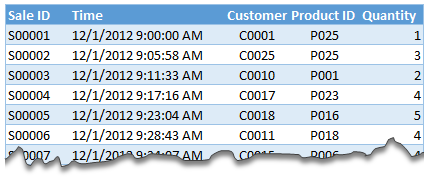
Lets say you are looking sales data for your company. You have transaction data like below.

Example data

And you want to find out how many units you are selling by product category and customer’s gender.

Unfortunately, you only have product ID & customer ID.

With VLOOKUP Hell,

  1. You first fetch all the customer and product data and place them in separate ranges.
  2. Then write a vlookup formula to fetch product category, another to fetch customer gender.
  3. Then fill down the formulas for entire list of transactions.
  4. Now make a pivot table.

Assuming you have 30,000 transactions, you have to write 60,000 VLOOKUP formulas to create this one report!!!

With Data Model heaven,

  1. Create relationships between Sales, Products & Customer tables
  2. Create a pivot table

Creating a relationship in Excel – Step by Step tutorial

  1. Relationship feature in Excel 2013 data ribbon tab
    First set up your data as tables. To create a table, select any cell in range and press CTRL+T. Specify a name for your table from design tab. Read introduction to Excel tables to understand more.
  2. Now, go to data ribbon & click on relationships button.
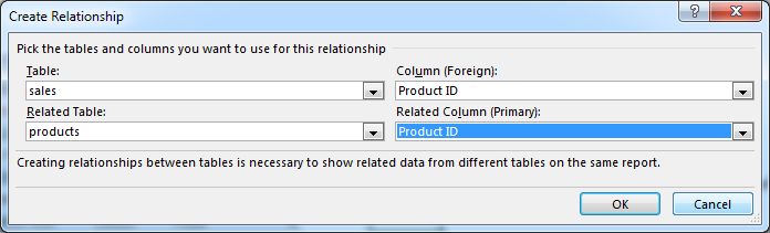
  3. Click New to create a new relationship.
  4. Select Source table & column name. Map it to target table & column name. It does not matter which order you use here. Excel is smart enough to adjust the relationship.
    Creating a new relationship in Excel 2013 - how to?
  5. Add more relationships as needed.

Using relationships in Pivot reports & analysis

  1. Select any table and insert a pivot table (Insert > Pivot table, more on Pivot tables).
  2. Make sure you check the “Add this data to data model” check box.
    Adding a pivot table with data model in Excel 2013
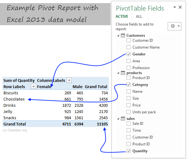
  3. In your pivot table field list, check “ALL” instead of “ACTIVE” to see all table names.
  4. Select fields from various tables to create a combined pivot report or pivot chart

Example: Category & Gender Sales Report

  1. Add category to row labels
  2. Add gender to column labels
  3. Add quantity to values
  4. and your report is ready!
Example Pivot report made with Excel data model

Things to keep in mind when you using relationships

  • Same data types in both columns: Columns that you are connecting in both tables should have same data type (ie both numbers or dates or text etc.)
  • One to one or One to many relationships only: Excel 2013 supports only one to many or one to one relationships. That means one of the tables must have no duplicate values on the column you are linking to. (for example products table should not have duplicate product IDs).
  • You can add slicers too: You can slice these pivot tables on any field you want (just like normal pivot tables). For example, you can further slice the above report on customer’s profession or product’s SKU size.

Benefits of Data Model based Pivot Tables

Once you have a data model in spreadsheet, you will enjoy several benefits (apart from multi-table pivots that is). They are,

  • Distinct counts: This simple but often tricky to calculate number is easy to get once you have data model based pivot. Just go to value field settings and change the summary type to “Distinct count”. Here is a tip explaining how to get distinct counts in Excel pivots.
  • Measures & DAX: Once you have a Data Model, you can unleash the full Power Pivot features on your workbook. You can create measures (using DAX language) and calculate things that are otherwise impossible with regular Excel. Here is an example of percentage of something calculation with DAX & Data Model, to get started.
  • Pivots from data in other files & databases: You can combine data model with the abilities of Power Query to create pivots from data in other places. For example, you can make a pivot from sales data in SAP with customer data in CRM system. Here is an overview of what is Power Query?
  • Pivots from more than 1mn rows of data: You can connect to very large datasets and make pivots from them with the help of data model. Here is a demo of how to set up data model for 1+mn rows of data.
  • Convert Pivot Tables to formulas: Once you have a data model based pivot table, you can turn it in to a set of formulas. You can access this feature from “Analyze” ribbon. This will replace your pivot with a bunch of CUBE formulas. Here is an overview of CUBE formulas.

Drawbacks of Data Model:

Of course, its not all cup cakes and coffee with Data Model. There are a few drawbacks of data model based pivot tables.

  • Compatibility: Data model & relationship feature is available only in Excel 2013 or above. This means, you cannot create or share such pivot reports with people using older versions of Excel.
  • Not able to group data: In regular Pivot Tables, you can group numeric, data or text fields. But with data model pivot tables, you can no longer group data. You must create another table with the group mapping and use it as a relationship.

Download Example File

Click here to download Excel data model demo file. It contains 3 different tables and a combined pivot report (with slicer) to show you what is possible.

Do you use relationships?

Ever since discovering PowerPivot, I kind of stopped using VLOOKUP (or XLOOKUP) for most of my own analysis. Now that relationships are part of main Excel functionality, I am using them even more.

What about you? Are you using relationships & data model in Excel? What cool things are you doing with it? Share your tips with us using comments.

Want even more? Try PowerPivot

If you want even more out of your reports, then try PowerPivot. It is a new feature in Excel 2013 (available as add-in in Excel 2010) that can let you do lots of powerful analysis on massive amounts of data. Here is an introduction to PowerPivot.

Facebook
Twitter
LinkedIn

Share this tip with your colleagues

Excel and Power BI tips - Chandoo.org Newsletter

Get FREE Excel + Power BI Tips

Simple, fun and useful emails, once per week.

Learn & be awesome.

Welcome to Chandoo.org

Thank you so much for visiting. My aim is to make you awesome in Excel & Power BI. I do this by sharing videos, tips, examples and downloads on this website. There are more than 1,000 pages with all things Excel, Power BI, Dashboards & VBA here. Go ahead and spend few minutes to be AWESOME.

Read my storyFREE Excel tips book

Overall I learned a lot and I thought you did a great job of explaining how to do things. This will definitely elevate my reporting in the future.
Rebekah S
Reporting Analyst
Excel formula list - 100+ examples and howto guide for you

From simple to complex, there is a formula for every occasion. Check out the list now.

Calendars, invoices, trackers and much more. All free, fun and fantastic.

Advanced Pivot Table tricks

Power Query, Data model, DAX, Filters, Slicers, Conditional formats and beautiful charts. It's all here.

Still on fence about Power BI? In this getting started guide, learn what is Power BI, how to get it and how to create your first report from scratch.

129 Responses to “Write a formula to check few cells have same value [homework]”

  1. Arie says:

    =NOT(STDEV(A1:A4))

    this also works for large ranges of numerical values (but not for text)

  2. Detlef says:

    Hi

    Works for numbers, text and logical values on a range from A1:An.

    =COUNTIF(A1:An,A1)=ROWS(A1:An)

  3. lockdalf says:

    well if you name the range, you could use following:

    =IF(SUMPRODUCT(1/COUNTIF('range','range'))=1,1,0) 

  4. Chris says:

    My solution is a, perhaphs slightly complex, array formula as follows:

    {=IFERROR(AVERAGE(IF(ISBLANK(A1:H1),9999,SUBSTITUTE(A1:H1,A1,9999)*1))=9999,FALSE)}

    Assuming there is a value (numerical, text, logic etc) in cell A1, this formula will work - and it will 'ignore' any cells that are 'blank' within the range A1:H1 (which can be extended to the required size).

    Breaking the formula down, the SUBSTITUTE(A1:H1,A1,9999) replaces all values (be it text / numerical) in the range A1:H1 that MATCH the value of cell A1 with the number 9999 (this should be changed to any number that WON'T APPEAR IN THE RANGE).

    These values are then multiplied by 1 (as SUBSTITUTE results in a text answer).

    Wrapping this in an IF(ISBLANK(A1:H1),9999,.........) formula takes care of any blank cells, setting them to this default value of 9999 also - this allows you to set the formula up once for a large range and then not have to alter as more data comes in.

    An Average is then taken of all these values - if all cells that contain values are the same, the average will come back to 9999.

    If all values are numerical but some differ, the average will differ from 9999 and will result in a FALSE answer. If some / all of the values are text and some differ from that in cell A1, the AVERAGE function will result in an Error, but in these instances the Match needs to return FALSE, hence the IFERROR function.

    Sure there's a simpler way to do this though!!

  5. George says:

    `{=IF(AND(COUNTA(RANGE)-SUM(--ISNUMBER(FIND(UPPER(FIRST ELEMENT IN RANGE),UPPER(RANGE))))=0,LEN(FIRST ELEMENT IN RANGE)=MAX(LEN(RANGE))),TRUE,FALSE)}`
    so if your data was in Column 1 and began in A1, you'd use
    `{=IF(AND(COUNTA($1:$1)-SUM(--ISNUMBER(FIND(UPPER($A$1),UPPER($1:$1))))=0,LEN($A$1)=MAX(LEN($1:$1))),TRUE,FALSE)}`

    This will work for strings and things, if you want it to be case sensitive (I don't), just remove the UPPER() part.
    What this does:

    `COUNTA($1:$1)`
    tells you how many entries you're looking at over your range (so we can work with an undetermined size).
    `--ISNUMBER()`
    ISNUMBER will return TRUE or FALSE depending on if the value inside is a number or not.  the -- part converts TRUE/FALSE in to 1 or 0.
    `UPPER()` OPTIONAL
    converts the value in to upper case.  If passed a number it changes it to text format.  This is what stops it from being case sensitive.
    `FIND($A$1,$1:$1)`
    will return a number if A1 is contained in each cell containing an entry in column 1.
    `LEN($A$1)=MAX(LEN($1:$1)`
    checks that all elements are the same length.  This is needed to avoid partial matches (without it, if A1 contained zzz and A2 contained azzza it would flag as true).

    REMEMBER this is an array formula, so enter with ctrl+shift+enter.

  6. Udit says:

    {=MIN(--(A1=OFFSET(A1,,,COUNTA(A1:A4))))}

    Gives 0 if false and 1 if true

  7. Ray Blake says:

    =COUNTIF(A:A,A1)/COUNTA(A:A) = 1

    This meets both bonus requirements and is dynamic. Keep adding more contents in column A and it will include these automatically. 

    • Mike K says:

      I like this a one a lot. I would make one small change by inserting a table for my data range. Makes it dynamic without selecting the whole column

       =IF(COUNTIF(tableName[colName],A2)/COUNTA(tableName[colName])=1,TRUE,FALSE)

  8. Sudhir Gawade says:

    For only Numeric values

    =MAX(A:A)=MIN(A:A)

  9. Sandy Siegel says:

    =(A1=B1)*(B1=C1)*(C1=D1)

  10. Elias says:

    Case sensitive.

    =SUMPRODUCT(0+EXACT(A1:A4,A1))=COUNTA(A1:A4)

    Regards

  11. PPH says:

    I'd use this

    =COUNTIF(range,INDEX(range,MODE(MATCH(range,range,0))))=COUNTA(range)

    It takes Hui's formula but ensures that the test value for the countif is the value or string that is most common in the range. Just in case you get a false but the problem is just with your test value being the odd one out.

  12. José Lôbo says:

    =SE(E(A1=A2;A1=A3);SE(E(A1=A4;A2=A3);SE(E(A2=A4;A3=A4);"ok")))
     
    SE = IF
    E = AND

  13. Stan Cullerne-Bown says:

    Bonus question 1 & 2
    Array formula: {AND(A1=A1:AN)}
    This will test all cells in range, including text and numbers. 

    Cheers 

  14. D Stinson says:

    A very simple solution uses Excel's Rank function.  Insert in B1 = Rank(A1, $A$1:$A$4).  Copy down this formula to B4.  If the answers in B1 thru B4 are all 1, the values are equal.  For an open range of cells, label the range of input (example "TestData") and place the label in the funtion (= Rank(A1, TestData) then copy down to an equivelent length of rows as the range.

  15. Tom Moedl says:

    =IF(SUM(A1:A4)/COUNT(A1:A4)=A1,TRUE,FALSE)

  16. Melanie says:

    =IF(SUM(A1:D1)/4=A1,"True","False")

  17. Tom Moedl says:

    I enjoy your emails.  I have learned a lot from them.  Thank you for what you do.

  18. .
     
    {=PRODUCT(--(A1=A1:A4))}
     
    .
    Change A4 to An.

  19. jimmy says:

    =IF((SUM(A1:A4)/COUNT(A1:A4))=A1,"TRUE","FALSE")

  20. Kishore Kumar says:

    I would use the formula which is mentioned below:-

    =IF(PRODUCT($A:$A)=A1^(COUNTIF($A:$A,A1)),"Yes","No")

  21. Karl says:

    At last a homework assignment that I could answer on my own. And I even understand some of the elegant answers from other readers this time.
    My solution was to nest IF statements:
    =IF(A4=A3,IF(A3=A2,IF(A2=A1,TRUE,FALSE),FALSE),FALSE)
    This satisfies bonus question 2 but I think the structure makes it impossible to modify this solution to satisfy bonus question 1. And I wouldn't want to use this strategy to compare very many values...

  22. Bob Bonner says:

    This answers all of your questions:

    =PRODUCT(--(INDIRECT("$A$1:$A$"&$B$1)=$A$1))

    where column A contains the values and $B$1 has the number of rows to assign to last A-cell. 

  23. Sanjay says:

    =IF(A1=A2:A2=A3:A3=A4>1,"TRUE","FALSE")
    =IF(A1=A2:A2=A3:A3=An>1,"TRUE","FALSE")
    =SUM(HELLO, A1)

  24. Livigs says:

    {=IF(SUM(IF(A1:A4=A1,0,1))=0,TRUE,FALSE)}
     
    This will work for numbers or text, and will work for any number of cells (A4 would just be An)

  25. Brian LaGrand says:

    Here's another alternate, assuming values in cells a1:d1
     
    =IF((A1*B1*C1*D1)^(1/COUNT(A1:D1))=AVERAGE(A1:D1),1,0)

  26. Supertaitai says:

    {=IF(AND($A$1:$A$4=OFFSET(A1,0,0)),1,0)}

  27. Virginia says:

    =SUM(IF(FREQUENCY(MATCH(A1:A4,A1:A4,0),MATCH(A1:A4,A1:A4,0))>0,1))

  28. Sanjay says:

    REVISED FORMULA
       =IF((A1=A2)*AND(A1=A3)*AND(A1=A4),"TRUE","FALSE")

    Regards

  29. Don says:

    =IF(SUMPRODUCT(--(A2:A5=A2))/COUNTA(A2:A5)=1,1,0)

  30. Bryan says:

    I would use something like this:  =COUNTA(A1:A4)=COUNTIF(A1:A4,A1)

    • Bryan says:

      You can even do a whole range and as you enter data into the range it tells you if they all match.  Going down to row 5000:  =COUNTA(A1:A5000)=COUNTIF(A1:A5000,A1).

      Thanks,
      B

  31. Manoj says:

    {=SUM(--(A1:A101=A1))=(COUNTA(A1:A10)+COUNTBLANK(A1:A10))}

  32. Ken ?-del says:

    For numeric values:

    =(OFFSET(list,,,1,1)=AVERAGE(list))

    where list = A1:A4 

    • Ken says:

      I need to retract my own post here guys. 

      It is WRONG! Let me explain.

      Suppose we have

      A1 = 1
      A2 = 0
      A3 = 2

      then Average = 1 and OFFSET(list,,,1,1) = 1
      so 1 = 1 but all the elements are NOT equal.


  33. Manoj says:

    correction 
    {=SUM(--(A1:A10=A1))=(COUNTA(A1:A10)+COUNTBLANK(A1:A10))}

  34. Pavel Lasák says:

    =IF(A1=B1,IF(B1=C1,IF(C1=D1,TRUE,FALSE),FALSE),FALSE) ....

  35. Matthew Holbrook says:

    =COUNTIF(OFFSET($A$1,0,0,COUNTA($A:$A),1),$A$1)=ROWS(OFFSET($A$1,0,0,COUNTA($A:$A),1))

  36. Parin Thacker says:

    I have a little more flexible approach. Suppose the value of 'n' is known. There is a possibility that only some of the cells in a row are filled up. For example if n = 10, then in a row, A1 to A10 must be compared. But in case only cells upto A7 are filled up. The formula thus has to adapt accordingly. Below formula does that:

    =COUNTIF(INDIRECT(ADDRESS(ROW(),1)&":"&ADDRESS(ROW(),COUNTA(A1:J1))),A1)=COUNTA(INDIRECT(ADDRESS(ROW(),1)&":"&ADDRESS(ROW(),COUNTA(A1:J1))))

  37. Ingo says:

    In A1:A100 is word/number
    In B1 is word/number we look

    C1=MAX(FREQUENCY(IF(A1:A100=B1,ROW(A1:A100)),IF(A1:A100<>B1,ROW(A1:A100))))  array formula

  38. Shubhro De says:

    We can use an array formula
    {=PRODUCT(--(A1:An=A1))}
    OR if we want n variable
    {=PRODUCT(--(INDIRECT("A1:A"&COUNTA(A:A))=A1))} 

  39. Steve LeLaurin says:

    {=AND(A1=A2:An)}

  40. Ariel says:

    I would use this one (simlpe)

    =(COUNTA(A:A)=COUNTIF(A:A;A1))

  41. uri Weiss says:

    try this
    =MAX(A1:A4)=MIN(A1:A4)

  42. uri Weiss says:

    Olso try this
    {=SUM(RANK(A1:A10,A1:A10))=COUNT(A1:A10)}
    Please notice it is an Array Formula

  43. elnur says:

    Dear All,
    i used that formula
    {=IF(COUNTIF(A1:A4,A1:A4)=COUNTA(A1:A4),TRUE,FALSE)}

  44. andy holaday says:

    Love the variety of responses.

    =MAX(A1:A4)=MIN(A1:A4)
    and
    =COUNTA(A1:A4)=COUNTIF(A1:A4,A1)
    will return true if the input range has blank cells

    My personal fave is the array formula {=AND(A1=A1:A4)}. Short and sweet, and easy to read. Blank cells will tally as a mismatch.

    A close second is 
    =SUMPRODUCT(1/COUNTIF(A1:A4,A1:A4))=1
    which will throw an error if blanks are present. 


  45. mahesh says:

    =PRODUCT(B1:D1)=B1^COUNT(B1:D1)...will return TRUE or FALSE

  46. Prem Singh says:

     
    Dear Sir,
     
    My answer is =exact(a2,a1)

  47. jack corley says:

    =IF((a1=a2=a3=a4),1,0)

  48. Arshad says:

    Hello Chandoo,
    We can also use Conditional Formatting......

  49. Akash Khandelwal says:

    For Numerics..

    =SUM(A1:AN)/A1=COUNT(A1:AN)
    results in True/False.

  50. Manoj Gupta says:

    =AND(IF(A1=B1,1,0),IF(B1=C1,1,0),IF(C1=D1,1,0))

  51. sam says:

    =AND(A1=A2:A4) array entered
    Generic
    =AND(A1=A2:An) array entered

  52. shrivallabha says:

    =--(COUNTIF(A1:A4,A1)=COUNTA(A1:A4))
    will give value as 1 or 0

  53. James says:

    Hi there, here's a simple formula to determine not only whether all 4 cells (A1 --> A4) are equal, but also whether any of the cells are equal and identifies which cells they are ...

    =COUNTIF($A$1:$A$4,A$1)*1000+COUNTIF($A$1:$A$4,A$2)*100+COUNTIF($A$1:$A$4,A$3)*10+COUNTIF($A$1:$A$4,A$4)*1

    A result of 1111 means no cells are equal, 4444 means all cells are equal, 1212 would mean there are 2 cells the same & they are in A2 & A4, etc

  54. Lood says:

    =((A1=B1)+(A1=C1)+(A1=D1))=3

    Obviously doesn't cover bonus question 1, but does so for q2 🙂
     

  55. Abhishek says:

    If formula

  56. Shmuel says:

    =MIN(A1:A4)=MAX(A1:A4)

  57. Faez says:

    Try this formula

    =IF(COUNTIF(A1:A4,A1)-ROWS(A1:A4)=0,"True","Flase")

  58. Werner says:

    I used the Swiss knife of excel: SUMPRODUCT, works for numeric as well as for non-numeric cell content and A1:A4 is obviously easily changed to any range.

    =IF(SUMPRODUCT(--(OFFSET($A$1:$A$4,0,0,ROWS($A$1:$A$4)-1,1)=OFFSET($A$1:$A$4,1,0,ROWS($A$1:$A$4)-1,1)))=ROWS($A$1:$A$4)-1,TRUE(),FALSE())

    • roirraWedorehT says:

      All of the individual non-array formulas (didn't test the array ones) have one flaw or another - mostly specifically if all the columns are blank, the result would still be false.

      Another formula in the comments worked for these but didn't work for when all columns had "0.00" in them. My solution was to OR the two. If H3 through H149 have your values, then this is what worked for me:

      =IF(OR(COUNTIF(H3:H149,H3)=COUNTA(H3:H149),SUMIFS(H3:H149,H3:H149,1)=COUNT(H3:H149)),IF(H3="","Blank",H3),"")

      This solution puts "Blank" if all the rows are blank, otherwise, it puts whatever the value that's in all of the rows - "0.00" or whatever.

      Thanks for all the answers!

  59. Allan R says:

    I used a nested if statement which also showed, via the false message, the first instance of cells which were not equal for the cells a1 to a5.

    =IF(A1=A2, IF(A2=A3, IF(A3=A4, IF(A4 = A5, "True","False A4"), "False A3"), "False A2"))

  60. Shailesh says:

    Hi,

    First, let me begin by saying, I am a big fan of all your posts and read your emails, mostly on the same day as you send them. I have not replied as much as I wanted to.

    This is my first attempt at answering a question on your post

    I came up with a simple check which will test if all values in a range A1:An are same or not

    Assuming range you want to check is A1:A10,
    In Cell B1, insert the formula 

    =IF(COUNTIFS(A1:A10,A1)=COUNTA(A1:A10),"All cells are same","All cells are not same") 

    The idea I applied is counting total number of non-blank cells and then counting the number of cells which match cell A1. If these are same, then it means
    a) all cells have the same value! (All can be blank, then both counts will be zero)

    I am working on finding the range automatically 🙂

    Can extend this into VBA and use InputBox etc to generate some user interaction

    Thanks
    Shailesh 

  61. Chirag says:

    =IF(COUNTIF(A1:A4,A1)=COUNT(A1:A4),TRUE,FALSE)

  62. Rafaqat Ali says:

    For homework & Bonus Question 3

    =IF(AND(A1=A2,A2=A3,A3=A4),1,0)


  63. Christopher A says:

    =IF(SUMIFS(A12:A15,A12:A15,1)=COUNT(A12:A15),1,0)

  64. Sanjeev Sawal says:

    One possible solution could be =+IF(COUNTIF(A1:A4,A1)-COUNT(A1:A4)=0,1,0)
    where A1:A4 is data range which can be a dynamic range and the formula can be modified accordingly. 
    Rgds,
    Sanjeev Sawal

  65. I got the right result with this one:

    =IF(A1=B1;IF(C1=D1;IF(B1=C1;1;0);0);0) 

  66. SIVAKUMAR R says:

    =and(a1=a2,a1=a2,a1=a3)
     

  67. SIVAKUMAR R says:

    ANSWER FOR bONUS 1

    =MAX(A1:A10)-MIN(A1:A10) 

  68. VaraK says:

    =AND(A1:A3=A2:A4)..Confirm with Ctrl+Shift+Enter (As as array formula). Works well for Text values and large range of values as well.

  69. Istiyak says:

    suppose cells contain 2 values ==== Yes | no

    formula :
    1
    =counta(a1:a4)=countif(a1:a4,"yes")
    It will return True or False.

    2
    =IF((COUNTA(A1:A4)=COUNTIF(A1:A4,"yes")),"Same value","Mis-match")
    it will return Same Value OR Mis-match.

    Hope you like it.

    Regards
    Istiyak

  70. Suraj Nair says:

    Also can use this formula
    =IF(AND(A1=A2,A1=A3,A1=A4),"1","0")

  71. Antonio says:

    Let say the values are in the range $B$1:$E$1, then the formula is:

    If(sumproduct(--($B$1:$E$1=$B$1))=CountA($B$1:$E$1);1;0)

    Please check that:
    * $B$1 was used as pivot value and could be randomly selected
    * It works well if parenthesis is omitted for values "1" and "0"
    * This formula applies also to "n-values" and non-numeric values (text, logical, etc.)

    Regards,

  72. Jorrie says:

    Hi, first time trying to solve a probleme.
    New at this but really enjoying Chardoo.org

    Think the following will work in all 3 questions

    {=IF(SUM(IF(A1=$A:$A,1,0))=COUNTA($A:$A),TRUE,FALSE)}

    Regards

    Jorrie
         

  73. Ashok Variyani says:

    use below formula for to get True / False

    =COUNTA(A1:A4)=COUNT(A1:A4)

    and use below formula for to get {1/0} or {match / Mismatch}

    =IF(COUNTA(A1:A4)=COUNT(A1:A4),{1,0} or {match,Mismatch})

  74. [...] Last week in Write a formula to check few cells have same value [Homework], [...]

  75. Cristian says:

    Hi, sorry if it's repeated, this array formula works well with numbers or text, the range can easily be dynamic: {=AND(A1:An=A1)} Now, after three days, I understand a lot more about array formulae, thanks?

  76. Adam says:

    =IF(AND(A1=A2,A2=A3,A3=A4),"TRUE","FALSE")

    • Yani says:

      What if there are not only four cells to compare but An?
      how will I determine if there is one cell that is not equal from any other cells?

  77. Netaji Bhopale says:

    =IF(COUNTA(A1:A4)=COUNT(A1:A4),1,0)
    =IF(COUNTA(A1:A4)=COUNT(A1:A4),”Match”,”Mismatch”)+
    =IF(AND(A1=A2,A2=A3,A3=A4),”TRUE”,”FALSE”)

  78. Aniket says:

    =iF(AND(EXACT(C15,D15),EXACT(E15,F15)),"Match","Mis-match")

  79. frank says:

    how this formula works in excel (B4+E4)/50*20
     

  80. Jerome says:

    I'm a little late to the party, but I figured I'd post anyways.

    For numbers only:
    =NOT(VAR.P(A1:An)) 

  81. nazmul_muneer says:

    The formula given below will fulfill the all criteria including bonus questions

    =IF(COUNTA(A:A)=COUNTIF(A:A,A1),"True","False")

    REGARDS 

  82. venkat says:

    =IF(MATCH(A1,A2:A4,0),TRUE,FALSE)
     

  83. Naveen Kumar says:

    =IF(COUNTIF($A$1:$A$4,A1)>1,"true","false")
    =IF(COUNTIF(A:A,A1)>1,"true","false")
     

    • Hui... says:

      @Naveen
       
      You can simplify your formulas as below:
      =COUNTIF($A$1:$A$4,A1)>1
      =COUNTIF(A:A,A1)>1
      Excel will return True or False without the need for the If() function

  84. Raghavendra says:

    Hi ,
     
    This question is similar to the one in the post.
    I have Text values in cell A1 and A2. 
    If A1 = A2, update 10 in cell A3 , else 0.
    Is there any formula for this. I am new to VB and hence do not have much knowledge. Eager to learn!!
     
    Thanks in advance !!!

  85. sandeep sharma says:

    =AND(A1=A2,A1=A3,A1=A4)

  86. sandeep sharma says:

    also =IF(AND(A1:A4=A1),TRUE,FALSE)

  87. Akshay says:

    One can use "IF, AND" formula.

    =IF(AND(A1=A2,A2=A3,A3=A1),"True","False")

  88. Cards says:

    =COUNTIF(A:A,A1)=COUNTA(A:A)

  89. Ritesh says:

    Enter array formula like, = IF($B$16:$B$21=$B$17:$B$22,"Yes","No")

  90. sunil gupta says:

    =IF(AND($E$5=$E$6,$E$6=$E$7,$E$7=$E$8),"true","flase")
    it can work try this one

  91. Andy Gore says:

    A question for you
    sheet 1 table A1:C10

    What formula in sheet 2 A1 will give me what is entered in the table sheet 1 A1:C10
    There is usually only one entry made in the table but if you can supply the answer to 1 or 2 entries I would be grateful

  92. Duncan says:

    =max(A:A)=min(A:A)

  93. Eduardo says:

    FOR TEXT DATA
    =COUNTIF(A1:A5,a1)=COUNTIF(A1:A5,"*?")

    FOR VALUE DATA
    =COUNTIF(A1:A5,A1)=COUNTA(A1:A5)

    Both Return TRUE or FALSE

  94. kaushik says:

    =if({sum(1/countif($A$1:$A$n,A1:An)}=1,"All Same","Not All Same")

  95. manish gupta says:

    I use formula A1=B1 and get value of TRUE / FALSE in C1. I had dragged this formula for 10 rows. Now in cell D2 i tried to put formula..

    =if(and(c1="False", c2="true"), "conflict", "no conflict")

    but even when the condition is true i am still getting no conflict.

    Can you please advice?
    thanks,
    Manish

    • Hui... says:

      @Manish
      Remove the " from around True and False
      =if(and(c1=False, c2=True), "conflict", "no conflict")

      In C1 and C2 you have a Boolean expression and it evaluates as True/False
      These are not text, although they do appear as Text, they are not 1/0 although they sometimes behave as 1/0, they are in fact Boolean values True/False

      So in your example you can simplify it as
      =If( And( Not(C1), C2), "conflict", "no conflict")

  96. Mohammed says:

    =SUMPRODUCT(MATCH(A1:A4,A1:A4,0))=COUNTIF(A1:A4,A1)

  97. adivyom says:

    Answer to both bonus questions 2 and 3:

    =COUNTIF(A1:An,A1)=COUNT(A1:An)

  98. Yves S says:

    answer to all questions:
    ={IF(ISERROR(MATCH(FALSE,((A1:An)=$A$1),0)),"same","different")}

    this works with numeric, non-numeric, and blanks:

    COUNT will not count numeric
    COUNTA will count blanks as one

  99. cnestg8r says:

    =SUMPRODUCT(1/COUNTIF(B1:J1,B1:J1))

    This will tell you how many unique values exist in the selected range. Text or numeric mixed.

  100. RAJIV SIROHI says:

    {=IF(AND(A1:A9=A2:A10),"EQUAL","NOT EQUAL")}

    this is an array formula, insert it with CSE.

  101. Anonymous Coward says:

    COUNTA/UNIQUE

  102. Tiago Couto says:

    =SUMPRODUCT(A:A)/A1=COUNT(A:A)

  103. Gabe says:

    =COUNTIF(A1:A4,A1) = COUNTA(A1:A4)

Leave a Reply