
Most of you know that during day time I work as a business analyst. Today while preparing some test scenarios for our latest insurance application, I came across a weird problem.
There are some steps in testing. For each test scenario, a combination of these steps is required. It is my responsibility to identify the steps as well as their combinations for each of the scenarios. So I quickly prepared a table with all the steps in left most column and one scenario each in one column. I put “X” in a cell if the step needs to appear in that scenario. But when I gave it to our testing team, they asked me if the scenarios can be explained a little better. See this picture to understand what they want and what I made.

So I immediately converted the “X”s to actual step names using a simple IF formula. (Copied the table, and wrote ‘if there is an X in the previous table, get the actual step from left most column otherwise empty‘).
Then the problem of actually removing various blank cells. First I tried to select all the blank cells and remove them using our technique from last week. But it failed as the blank cells are actually formulas with empty values. So I copy pasted the entire table as values (CTRL+C, ALT+ESV). But even then excel wont recognize blanks as true blanks (because the value is actually “” instead of being plain empty.)
Now I didnt want to manually select all the blank cells as the real testing scenario table had 50 scenarios with 68 possible steps.
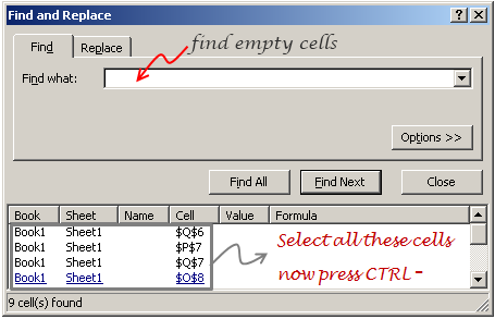
Then it stuck me, why not use FIND (CTRL+F) to find all the cells containing nothing? So I selected the scenario table, opened the find and looked up all the cells that contain empty values. Now I clicked on “Find all” and selected the entire list of values from that. Finally I removed all these cells and bingo!
PS: Our testers was more than happy as it took very little time and they had all the scripts ready.
PPS: Thanks to Rick, who taught me FIND ALL approach to select blank cells (here).


17 Responses to “Find and Remove Blank Items from a Range of Cells [personal experience]”
Great tip!
I often don't trust the find function as I sometimes don't consider all the implications. Often times when I need to create 'real' blank cells I just use text to columns.
If you select text to columns then click finish (providing you've not done any converting before hand) it will delimit by tab, which you dont have any of and re-process the cells which leaves you with some beautifully empty cells.
I am curious....what happened to steps 4, 8, and 9? They did not move to the second table.
@Camping.. my bad. I made a mistake in the illustration. Didnt realize it until now. I will fix and upload a new image.
@Paul: very good suggestion 🙂
@Camping.. now it is corrected. Thank you for pointing it out 🙂
Thanks teacher.....I shall send you another apple.....one less pixely this time.
The find and replace method is also useful for imported data when deciphering between "soft spaces" (Char32) and "hard spaces" (Char160), or get around it using IF and SUBSTITUTE formulas.
Great tip.
You could use Goto (Ctrl+G) > Special > Blanks to find blanks in your pasted-special range.
In the formulas, if you put =na() instead of "" for the false condition, you get some cells with #N/A. Then you can use Goto (Ctrl+G) > Special > Formulas, uncheck all except Errors to find these cells and delete them without changing the formulas. Of course, in this case, the formulas are useless by this point.
Hi Chandoo,
thanks for changing the subject line of your e-mails. I always used to change it based on the content you were sharing in order to easy find the correct one in case I needed some help. But know I don't have to do that anymore, perfect and much appreciated 🙂
Hi Chandoo,
I've just 'unsubscribed' from your newsletter/RSS Feed because I am leaving my current job, but don't be sad because I have re-subscribed with my own email address and also signed up my colleague! Lose 1 gain 2! My colleague will find this site very interesting and helpful going forward - especially as I will not be around to help anymore.
@Jared and Jon: good tips 🙂
@Anne: You are welcome. Thanks to the folks at Feedburner for allowing this option on email newsletters.
@Cape: Are you joining another job or working on your own now? Thanks for recommending the site to your colleague.
A little bit of both Chandoo. I've a small business that I intend to build up and I'm available for part time work to keep me out of trouble and ofcourse keeping up with your site.
You're very welcome on the site recommendation. I never miss the opportunity to pass your details on.
On the latter, I'd like to ask permission to put a link on my site pointing to yours? If you are in agreement, do you have a banner I could use or would you prefer I just put a link - something like the links in the 'Ads by Google' section you have?
I can relate to "Excel doesn't see the "" as blanks" fight.
I overcame it by using either a number value or a text value in my IF statement,
depending on the nature of the other value.
Now I can use the GoTo Special, select Formulas with Numbers, and DELETE!
-->
if there is an X in the previous table,
get the actual step from left most column
otherwise
(And of course, if the values being brought in were numeric, use )
Thanks for the tip
Please Help
what is the formula for replacing "X" value
Regards
[...] Find and Remove Blank Items from a Range of Cells [personal experience] » [...]
FANTASTIC. THANKYOU VERY MUCH FOR POSTING THIS.
HELP!
I tried posting a minute ago but wasn't registered, sorry.All registered now.
I've created a monster...a series of worksheets for managing a hotel's reservations and guest information. I have 12 main sheets (one for each month) with areas for each day of said month and space for 24 possible reservations on each day (we have 24 rooms).
So january has potentially 31 x 24 reservations.
Put all of the months together and I have another worksheet that looks at all the others and selects the information for reservations if there are any. This worksheet has 9127 rows... I kid you not. I am self-taught and not long in the game and I'm sinking with this problem.
What I want to do is remove all of the blank cells (rows) from the huge worksheet and put the info remainnig into another worksheet that displays only actual bookings. I've used an IF formula for the huge worksheet to only supply data or return "" if not.
We don't have bookings every day and we rarely sell 24 rooms in a day so most of the 9127 rows are blank. I want a way to remove the blanks and display the actual reservations. I've tried "NoBlankRange" formulas, your earlier suggestion of FIND and nothing works. I'm using excel 2007 and need help. I can supply a copy of the spreadsheet if you need to see it, but generally I'm just after some options or perhaps advice on how to proceed.
I hope someone can see where I have gone wrong 🙂