
 Today I have learned this very cool way to find if a list has duplicate items or not.
This technique uses array formulas (do not shudder, believe me they are not as difficult as you may think)
First the formula
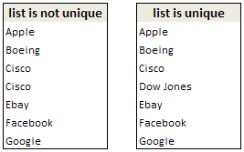
Assuming your list is in the range, C3: C9, the array formula to find if a list has duplicate items or not is,
=IF(MAX(COUNTIF(C$3:C$9;C3:C9))>1,"list is not unique","list is unique")
Now the explanation
How do you know if a list has no duplicates? Simple, we find the number of times each item has appeared in the list and see if any of those counts are more than 1.
Now, take a look at the formula. It says find the maximum of individual item counts using countif (learn excel countif function) and if the maximum is more than 1, then the list has duplicates, otherwise it is unique.
But…
Yes, entering the formula will not work by itself. You have to make it array formula.
How do you do that?
Oh, that is simple, you just take the excel spreadsheet and whack it until it turns blue.
well, not really. all you need to do is enter the formula and press CTRL + SHIFT ENTER instead of just pressing enter.
that way excel converts your formula to array formula and the COUNTIF(C$3:C$9,C3:C9) will return an array of counts instead of one value. Now you can also guess why we have absolute reference for one parameter of countif () and relative reference for another. Learn more about Absolute and Relative References in excel formulas.
More on Finding and Removing Duplicate Items
> Using pivot tables to get unique items in excel
> Getting unique items using data filter and formulas
> Use advanced data filters to find unique items
> Eliminate Duplicate Entries in a List using Formulas
> Get Unique items using Excel 2007 built in features
This post is part of our Spreadcheats series, a 30 day online excel training program for office goers and spreadsheet users. Join today.


54 Responses
Hello Mr Chandoo!
Could you double check the formula you have provided. I am getting an error – Excel will not accept the formula =IF(MAX(COUNTIF(C$3:C$9;C3:C9))>1;”list is not unique”;”list is unique”) – It seems to be having a problem with C$9 part of the formula.
Many thanks PHD. Appreciate the time you give to this website.
denise
Denise,
I guess Chandoo is using an European installation of Excel at the moment. If you are using an English version, you have to replace the “;” by “,”.
Ah – Thank you Robert. That’s very kind of you to reply so promptly. And you are right – it now works with “,”
Cheers Robert. All the best to you.
Denise
@Denise, as Robert pointed, I have been using European version of excel which uses ; to seperate formula arguments instead of comma. So when I copy pasted the formula from my test workbook, I forgot to change the semicolon back to comma. I have corrected the post now.
@Robert: Wonderful guess and thanks 🙂
Chandoo,
Thanks for a great blog. I have gone through all the posts on duplicate but the issue I have is that the duplicates are not named in the same way. For example:
ADT Security
A D T Security
are both the same but was entered differently (one with space and one without space). How do I go about this? I have 8000 rows of data I need to identify duplicates that are mostly nonidentical.
Thanks for your help!
Welcome to Chandoo.org Cindy. Thanks for the comments.
If you have only extra spaces, then you can use something like =substitute(value,” “,””) and then lookup in them to see if there are any duplicates.
But if you have some spelling mistakes and other, then you can use a small FUZZY match VBA function, as shown here:
http://chandoo.org/wp/2008/09/25/handling-spelling-mistakes-in-excel-fuzzy-search/
Here’s how I do it:
=IF(COUNTA(A1:C100)=SUM(1/COUNTIF(A1:C100,A1:C100)),”No duplicates”,”Some duplicates”)
Also, you can change your formula separator (in WinXP) by going to Control Panel, Regional and Language Optionsand click “Customize” near the top of the dialog box. Then you could change your list separator to ; and use Chandoo’s formula without alteration. But I wouldn’t recommend it 😉
This formula is lovely!!!
@ JP, true, there is often more than one way to get at a solution.
Arrays can be very a powerful though, and can often overcome shortcomings in other methods. Array formulae can do some truly amazing things and deserve much more press.
For example, suppose you have the following and you want the median Num of “A” Codes:
Code Num
A 6
B 10
C 12
A 16
B 32
C 15
An array takes care of this easily, and provides a solution where other methods do not exist:
=MEDIAN(IF(A2:A7=”A”,B2:B7))
The formula must be array-entered (Ctrl+Shift+Enter) to work properly, of course.
If we wanted Average we could use pivot tables. If we wanted Sum we could use a pivot or SUMIF. But for Median, there is no other convenient way. Moreover, to get Average or Sum, simply substitute those functions for MEDIAN and it is done.
HI Chandoo,
I have seen most of your blogs and has helped me in resolving most of excel formulas issues.
However, I have one issue which is bothering me from quiet a long time and I’m not getting a solution.
I’m counting on you and your blog members to help me resolving this.
What I Have : I have 2 columns. First with unique names and second column have numbers associated with the names (I’m taking example as above).
What I want : I need to highlight the Max Value (Second Column) against each Individual names.
Code Num
A 6
B 10
C 12
A 16
B 32
C 15
Output Should be :
A 16
B 32
C 15
AshP
Assuming the data is in A1:B7 and you have A, B , C in D1:D4
In E2: =MAX(IF($A$2:$A$7=D2,$B$2:$B$7)) Ctrl+Shift+Enter
Then copy E2 to E3:E4
You may wish to have a read of:
http://chandoo.org/wp/2012/01/24/formula-forensics-no-008/
Thanks a ton, Hui.
I have acheived the required results now.
well being an infant in excel knowledge i like to keep things simple so here is my simple formula
=IF(COUNTIF($A$1:$A$10,A1)>1,”duplicate”,”no duplicate”)
Can also Copy the column onto a new sheet, Pivot Table the column with the column on left side (row) and the “Count” of the column in middle (Data). Any duplicate row will be over 1 (can sort decreasing to see them in 1st)
I am trying to apply the principles of arrays included in this post to analyze the following real-world problem, but I have had no success. I’m wondering if someone can provide some guidance:
The goal is to count the number of unique (non duplicate) customers in any one month. The data looks something like this:
Customer Month Sale ($)
John apr 20
Brad apr 25
Ellen may 15
Ron jun 20
Toby jun 10
Toby jun 10
Juan jun 25
Brad jul 30
So for Apr the count should be 2 (Jon & Brad), for Jun the count should be 3 (Ron, Toby & Juan), and for Jul the count should be 1 (Brad).
I’ve been able to count unique customers (non-duplicates) in the entire list, but not unique customers by month.
Any help would be greatly appreciated.
-Rob
@Rob: Welcome to PHD and thanks for asking a question.
I like this problem very much, so when I got home from work I have spent sometime researching array formulas (and ended up learning a ton of cool stuff).
To count the month-wise uniques, you can use offset() formula. Ofcourse, this only works if the list is arranged month-wise. But probably that is not such a difficult task.
I have made one solution that works with offset and array formulas and uploaded it here:
http://chandoo.org/img/n/array-formulas-query.xls
Let me know if this doesnt work for you…
Thanks Ninja. But your formula returns 3 for the month of June while the answer is 4. Please check that. I have made this alternative formula: SUM(IF($C$3:$C$10=F3,IF(COUNTIF($B$3:$B$10,$B$3:$B$10),1)))
I withdraw my comment. I am sorry
This is a good problem and I happen to have a solution in my bag-o-tricks called “count unique items with constraint”.
Assume your data in A2:C9, and A12=”apr”, A13=”may”, etc.
This formula in B12 will return result for “apr”. It is an array formula that can be filled down:
=SUM(N(FREQUENCY(IF($B$2:$B$9=
A12,MATCH($A$2:$A$9,$A$2:$A$9,0)),MATCH($A$2:$A$9,$A$2:$A$9,0))>0))
The IF specifies the constraint. If you remove it you will get unique customers without regard to date.
=SUM(N(FREQUENCY(MATCH($A$2:$A$9,$A$2:$A$9,0),
MATCH($A$2:$A$9,$A$2:$A$9,0))>0))
These were highly instructional to me. If you use the “Evaluate Formula” tool and follow the evaluation steps very carefully you can learn lots about how array formulas work.
Thanks for a great formula. But it is returning 3 for the month of June. Instead of 4 which is the correct number. I wonder why
Hi Andy –
Thanks for the reply. I’d like to explore your solution further but I believe some of the formula was cut-off when your reply was posted (possibly a text wrap issue). is there any chance you can re-post the formula?
-Rob
Hi Rob, the rendering by the forum is unfortunate, but if you select my entire reply using the mouse and copy / paste to another viewer (e.g., notepad) the whole answer should be there.
Aside question to PHD… is there a better way to post long lines of code?
@Andy.. good formula.. I havent tested it yet…
my formula looked something like this: =SUM(1/COUNTIF(OFFSET($B$3,MATCH(F3,$C$3:$C$10,0)-1,0,COUNTIF($C$3:$C$10,F3)),
OFFSET($B$3,MATCH(F3,$C$3:$C$10,0)-1,0,COUNTIF($C$3:$C$10,F3))))
Also, to get unique count without any other conditions you can try the sum(1/countif(range, range))
here F3 has the month APR, C3:C10 has the months and B3 onwards the people list
Btw, you can enter long formulas by manually inserting breaks. This theme doesnt support super long text nor it does insert line breaks automatically. If it doesnt chop then the layout is screwed.
@Chandoo, thank you very much for your explanation about array formulas.
I downloaded the array-formulas-query.xls spreadsheet and I’m trying to understand how you got the single cell reference to increment in the array formula. I must be missing something simple.
Whenever I try to type in an array formula and use the Ctrl+Shift+Enter to enter it, it puts the formula in as an array formula, but it repeats the same value for the cell reference in every position of the array.
In other words if I try to enter just a portion of your formula above as =COUNTIF($C$3:$C$10,F3), it puts the exact same formula in every position of the array. Thus in your sample spreadsheet I get the count for “apr” in every row of the array.
@Kelly.. array formulas expect that you use a regular formula but with arrays instead of one value. the countif syntax is countif(range, filter-criteria). So when you enter something like this: =COUNTIF($C$3:$C$10,F3), it still works like a normal formula even though you enter it as an array formula.
where as this formula: =COUNTIF($C$3:$C$10,F3:F10) works like an array formula as excel calculates 8 different values (=COUNTIF($C$3:$C$10,F3),=COUNTIF($C$3:$C$10,F4), …, =COUNTIF($C$3:$C$10,F10)) when you press ctrl+shift+enter
I hope this is a bit clear now.. I suggest you to see more array formula examples to understand how they work.
http://chandoo.org/wp/tag/array-formulas/
Thank you for the clarification. Your explanations made sense so I took another look at your array-formulas-query.xls spreadsheet. I then realized that you put in four individual array formulas under the Unique customers column. I initially thought that they were a single array.
Thanks again for your excellent examples an explanations in the whole PHD site. I have learned quite a few things from your articles.
hi. i got to resurrect this cuz it’s driving me crazy 😀
assuming data is in A2:A10. target unique list is on B2.
i manage to get the unique list using this array formula: {=IFERROR(INDEX(A2:A10,MATCH(0,COUNTIF($B$2:B2,A2:A10),0)),””)} … but the list isn’t sorted.
how can i get the unique list from A2:A10 -> B2, and sorted (ascending)?
thanks!
Chandoo
Think I found a minor error on the page:-
http://chandoo.org/wp/2009/03/25/using-array-formulas-example1/
you used ; in the middle of
=IF(MAX(COUNTIF(C$3:C$9;C3:C9))>1,”list is not unique”,”list is unique”)
where my Excel was only happy with ,
Then it worked.
Keep up the good work. GREAT Site.
Nigel
@Nigel: I have a european excel version installed on my comp. It uses ; as the separator in formulas. I often forget to replace the ;s in the formulas with ,s when pasting them here. 😀
Thanks for your compliments.
@Cybpsych: Are you able to solve the problem. Let me know.
i needs formula for duplicate in excel.
Let’s assume that we have data on two columns ie. B and C. The data may repeat on the same column but should not on both columns. Our data range for this example is “B7:C19″. The formula to use in excel 2007 is:
=IF(COUNTIFS($B$7:$B$19,B7,$C$7:$C$19,C7)>1,”Duplicate”,””). Use this formula in D7 and copy to the row range in column D.
The formula to use in versions before 2007 is:
=IF(MIN(COUNTIF($B$7:$B$19,B7),COUNTIF($C$7:$C$19,C7))>1,”Duplicate”,””). Use this formula in D7 and copy to the row range in column D.
This is not an array formula and CSE is not required.
Duplicates with multiple criteria
The formula to use in versions before 2007 is:
=IF(MIN(COUNTIF($B$7:$B$19,B7),COUNTIF($C$7:$C$19,C7))>1,”Duplicate”,””) has some limitations. It does not work under some conditions.
We can instead use the following array formula:
Let’s assume that we have data on two columns ie. B and C. The data may repeat on the same column but should not on both columns. Our data range for this example is “B7:C19?
=IF(COUNTA($B$7:$B$19)-COUNT(IF($B$7:$B$19&$C$7:$C$19=B7&C7,B7&C7,0))>1,”Duplicate”,””)
Need Help with excel formula:
i have 2 columns, one column states the job status(such as planned, Unplanned, EMERGENCY etc) and other column states the date.
My question is, what would be the formal if i need to count Individual status for a particular months, so that i can tabulate it in below format..
PLANNED UNPLANNED EXTRA HIRE CALL OUT EMERGENCY SHUTDOWN EMERGENCY
January
February
March
April
May
June
July
August
September
October
November
December
@Suheb
I assume your data has two named ranges: Date and Status
I have a column January-December in Column: D3:D14
I have the status’s listed in Row: E2:K2
.
If your dates are in a single year then you can use something like:
=SUMPRODUCT((TEXT(Date,”mmmm”)=$D3)*(Status=E$2)).
If you have multiple years of data, try the following
=SUMPRODUCT((YEAR(Date)=Year)*(TEXT(Date,"mmmm")=$D3)*(Status=E$2)).
Where I have a Named Formula or cell called “Year” with 2011 in it
.
You will have to retype all the ” characters if you copy/paste these formula
I have a non-unique list of book names. Can I get the count of the uniqie book names with an ecel formulae?
@TANVI
Try this. If your list is a range called “Myrange”,
[code]
=SUM(N(FREQUENCY(MATCH(Myrange,Myrange,0),MATCH(Myrange,Myrange,0))>0))
[/code]
Note this is not an array formula.
I have a problem with vlookup and duplicates. if column A is product code and column B is quantity…column C to J is etc…. where product code can appear many times in the column with different quantities and etc…, how can I create a report on a separate sheet using vlookup or any other formula and get all the different rows with the same product code?
I have an excel spreadsheet of information where there are multiple columns. There are instances of duplicate rows based on the First and Last name columns, the information in the rest of the columns may be different; there is a unique iD column, the highest ID= the newest record for that name. I need to create a list of unduplicated records showing all the information from the list where the record pulled is the maximum Unique ID for the name. Can anyone help me with the formula?
I’m always looking for a formula that will find the duplicates in one column (like a customer number) and then look at a second column to find a unique value (like a specific part number), and then mark all lines of data for those customers, even the lines that don’t have the specific part number. That way I can see each line for that customer who bought the specific part, and still see the other parts they bought too.
Hi,
If Same column Data word is repeatedly coming then how to remove this word with formula, kindly sugest with example.
Like :- Subh Mon Mon (requirement is Subh Mon).
Thanks,
Subhankar
@Subhankar
Does =LEFT(A2,FIND(” “,A2,FIND(” “,A2,1)+1)) work?
Hi Hui,
It is not working 🙁 I am using on MSOffice2010
Like :- Subh Mon Mon (requirement is Subh Mon).
Thanks,
Subhankar
Hi Hui….,
My Data is like this :-
KITIMAT PL (Correct)
KITIMAT PL PL (here it is repet “PL”) with formula can remove ..?
KITIMATT PL
@Subhankar
Try:
=IF(LEN(A2)-LEN(SUBSTITUTE(A2,” “,””))=<1,A2,LEFT(A2,FIND(" ",A2,FIND(" ",A2,1)+1)))
You will have to retype the " marks as WordPress stuffs them up
Note there are spaces between some of the " marks
=IF(LEN(A2)-LEN(SUBSTITUTE(A2,"_",""))=<1,A2,LEFT(A2,FIND("_",A2,FIND("_",A2,1)+1)))
change the _ for spaces
Hi Hui,
Thanks..!!! it’s works but some of column deleting non duplicate also.
One more quiry, if same workbook in another sheet (sheet3) reference data search in Sheet1 for duplicate.
Example:- Sheet1 dat
A2 cell (or any ware of the sheet)- KITIMAT PL PL
sheet3 –
Any ware in that sheet – PL (search this PL in sheet1 and delete only last repert one not any midil of the name… etc)
please help me out….
Thanks,
Subh
@Subh
Can you please ask the question at the Chandoo.org Forums
http://chandoo.org/forums/
Please also attach a sample file with a sample of the desired output
hai chandu u r blog simply superb…,
I have a small querry for my requirment the que is
In a list of values i need a formula to sort and remove duplicates
Kindly give respond to my querry
Thanking u
Input:
A 12
A 11
A 10
B 11
B 12
Out put:
A 12 11 10
B 11 12
Hi All,
Need resolution ASAP,
I have duplicates in Column A, other values in B column ranging from 1-40. So what I need duplicates should be removed in Column A, but in B column should have only minimum values.
In a B column values started from 1, some are with 2 and few are with 3, so duplicate should be removed but other column should have only minimum value
A B
4473678 1
4473678 16
4473723 2
4473723 6
4474015 10
4474015 6
4474015 1
4474028 1
4474028 4
4474028 6
4474115 33
4474115 7
4474115 40
4474115 2
4474115 15
4474115 19
Excellent suggestion / solution. Found quite a number of other blogs/sites trying to solve the same problem, but none is as simple and clean as this.