
Reem, one of the PHD readers, asks in e-mail,
Is there a way to prevent users from unhiding “hidden sheets” in an excel file – without using VBA?
or to put it in other words, can the “Format/Sheet/Unhide” be disabled for specific worksheets?
Here is a non-VBA way to do this. I am not sure if this is optimum, but it seems to produce results without much effort. And it doesn’t use VBA, just the VBA Editor.
Step 1: Right click on the tab you want to hide and select view code option

Step 2: In the properties window for that sheet, set “visibility” as 2 – xlSheetVeryHidden

Step 3: Now right click on the sheet name in project explorer area and select VBA Project properties

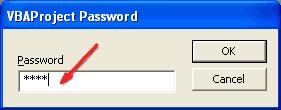
Step 4: Go to “Protection” tab and check “Lock” project

Step 5: and set password for protection, click ok

Step 6: when someone tries to open the VBA Code for that sheet to make the worksheet tab unhidden (visible), Excel prompts for a password
This trick is very handy when you are sharing workbooks with others and afraid that they may ruin the calculations or data.


78 Responses
It’s a —- ! Not to hide a sheet but to protect VBA……. This protection is very easy to destroy and it’s not a real protection… Try Acyd.xla to convince you… you will see !
To download Acyd.xla, google it !
@Souri: Welcome 🙂
I think you missed the step on changing the visibility to xlSheetVeryHide. Even if you do that and dont add VBA protection, you will be able to revert back the sheet by changing the visibility property. That is why you need to add VBA protection.
Of course, you can always break any type of protection using some crackware, that is not the point of this discussion though.
And, we would appreciate if you use a more acceptable language to share your enthusiasm.
How to see that sheet which i have made unvisible
@Honda
Right click on another Tab and Unhide
mine the unhide button goes grey. what shoul i do? please help
hi Chandoo, thanks for guiding us on excel. steps are superb just need to be used in daily use…
I tried your above procedure to hide a worksheet & i did it but unable to get back now. could you please advice me for the same.
Speaking of things you can (or can’t) do with an Excel worksheet tab; the other day I unconsciously reached for an affordance that wasn’t there. I was given a workbook with a confusing number of tabs on, so I thought “I know! colour coding them will make it easier to navigate” and went to change the colours of the tabs.
Of course Excel has no such capability, as I would have remembered if I wasn’t working in the morning before coffee. After all, Quattro Pro only had it twenty years ago.
Derek,
I might be misunderstanding your question, but as far as I know Excel lets you change the color of the tabs already since Version Excel 2002 (right click on the tab and choose tab color).
In Excel 2007, you can also disable that menu choice using RibbonX xml code. It isn’t secure, but the average user won’t have a clue how to unhide it.
Chandoo…
I have been visiting your blog for the past couple of months and I must say, it is superb. Each post is useful and I often use what you share at my work. Via your site, I have found quite a few other incredible excel blogs.
Next time you are in Bangalore, the coffee is on me. 🙂
Cheers,
D.
@Sumit, sweet.. free coffee. I might come to Bangalore in the next month or so for some work. 🙂
Oh, that’s good to know. Unfortunately I’ve only got 2000 at work. We were on the very brink of getting 2003 (not 2007!) when the recession hit and all our IT spending was cancelled.
Thank you Mr.Chandoo for giving many useful tips.I am so attached to chandoo.org,coz its beefing up my excel knowledge tank day by day.thanks a lot.
@Suryachandra: You are welcome 🙂
@Tim: that is very good to know. Thanks for sharing it with us. But if we disable the menu choice using RibbonX code and send the workbook to someone else, wont they be still having access to the menu choice.. ?
@derek: that means you have a stable version of excel at work for the next few years. no more wasting time with creating compatible versions and coping with new features.. 🙂
We were going to get a stable version. I was really impressed when I heard the upgrade was going to be to XP and Office 2003; I said “You can still get those!?”
That’s why I’m frustrated by the cancellation: we were so close to something that would stand good for many more years, and now who knows if we’ll be stuck with Vista and 2007 when the spending finally comes through? While everyone else moves on to whatever MS manages to salvage from the mess.
Hi Chandoo,
I have an excel which is suppposed to have 3 sheets, but at one time only one sheet is visible.
Also, I cannot see any tabs.How the heck do I unhide all the sheets, make them visible at the same time, and how the hell do I get my tabs back.
-Sindhu
@Sindhu: The excel workbook must be having “hide sheet tabs” option turned on. You can turn it off from excel options > Advanced options in excel 2007 or excel options menu item in excel 2003.
Also, it might be possible that the excel workbook has some macros which might be causing this behavior. In that case, turn off the macros and open the workbook again and you might be able to see all tabs.
I tried to set a pass for the code, but is not working. I´v tried on all of the sheets (7) on my workbook, I tried on the VBA project, but when i close and reopen, the pass is gone. And yes, i have save changes before closing.
Can anyone help me? Thanks.
@Liliana… which version of excel you are using? The tip has been tested in excel 2003.
Hi Chandoo,
The hide under format is grayed out and I’m unable to hide the sheet using the VBA.
it throws up an error like this Unable to set the Visible property of the worksheet class.
Please help
Chandoo,
I’m a newbie and plan to do much more exploring. Your explantion is clear and pictures are good. But…
Using Excel 2007 I get the same error as ‘Goofy’ when I try to choose 2-very hidden but that is because the VBA project listing window jumps to the next ‘higher’ tab – so I just choose the tab again in the Properties Sheet window. After I right click on the sheet in the VBA Project window and choose VBA Project Properites, it lets me check the lock box, and set a password but when another person tries to change it back to ‘visible’ it changes back without asking for a password.
I’ve played around with Excel Options/advanced/show sheet tabs, and display options for this workbook and nothing seems to make a difference.
Any insight into what I’m doing wrong
Hi,
How to create a dynamic row in a summarising sheet when a new sheet dynamically adds in a workbook
Hi, I used this process sometime back when my Office version is still 2003. This doesnt seem to work with version 2007. Do you have any idea why?
Thank you. I used this on my company. Thanks a lot.
Oh yes I have not tested it on 2007.
I can also use
select all rows to be protected in the sheet.
Then Hide the cells then.. Protect it.
So to see it must unprotect it then unhide the cells protected.
I believe I followed the steps outlined above, including saving the file, however after reopening it, I was able to access the properties of a tab and change the it back to “visable” with out being prompted for the password I previoulsy entered. Is there a step I’m missing such as saving the project? I’m not sure why I was able to change the properties without entering the password. Help
Dear TG,
That is the same thing I experienced. Chandoo, we need your help!!! It asks me for a password, I put one in, but aftyer I send it or slide it over to a shared folder on the company server other people can open it on their computer and chagne it to ‘visible’ without being asked for a password. I don’t think this way works in 2007. Microsoft screwed up! Chandoo, please help, or at least confirm what we suspect so we can move on and deal with this problem in another way. Thanks!!
How to view that protected sheet again
How to unhide and view the protected sheet again ?
@Asher
Unhide and Proetction are 2 different things but see below
.
To Unhide a sheet Right click on a Tab and Select Unhide, an Unhide dialog will appear, select the sheet to unhide and OK
.
To Unprotect, goto the Review, Unprotect Sheet Tab
Thanks Hui for coming back to me so quickly. I was not clear in my question.
I just did disabled -> Format/Sheet/Unhide , using the method decribed in the post, so now how do I go about getting the option enabled again.
@Asher
Format/Sheet/Hide
or Right Click on Tab and Hide
.
The Post is about using the Code Window Propperties to Set Hiden/unhidden properties
Right Click on Tab, View Code, Properties window for that sheet, set “visibility” as 2 – xlSheetVeryHidden etc
Mr. Chandoo,
Does this work in Excel 2007?
@Betsy
Yes it works in 2007/10
Hi Chandoo,
Can we disable / hide the properties of a Worksheet, in Excel 2007. The solution given by you above works fine in Excel 2003. I tried saving the file as xlsm also but not positive, it worked fine; but by creating a dummy procedure. Is there a solution where without having a dummy procedure I lock / disable the properties of the Workbook / Worksheet.
@Deepak, Betsy
This only works when saving the file as an .XLSM in 2007/10.
The whole idea is that you will have an UnHide subroutine to make the very hidden sheets visible and so locking the VB Editor makes it secure
@2007/2010 users, Hui is right. It does work on those versions but you have to make sure its a macro-enabled type of file (.xlsm) and not the regular excel file type (.xlsx). This is to confirm that it still works in 2007 & 2010.
@Chandoo, thanks for sharing this. Will be adding your site as one of my references from now on.
Now that I have hidden a worksheet, how do I unhide it?
@Kmnegast
Right click any sheet tab and View Code
Find and select the hidden workbook/sheet in the VBA Project Window
In the Properties Window set visible to -1 – xlSheetVisible
.
or
.
Right click any sheet tab and View Code
Click in the Immediate Pane
type
sheet2.Visible=xlSheetVisible
Change Sheet2 to the name of your hidden worksheet
@ Chandoo & Hui
Sorry guys but i tried this in both a normal workbook and a macro enabled workbook in 2007 but it doesnt seem to work
Any suggestions ?
@2007/2010 users, Hui is right. It does work on those versions but you have to make sure its a macro-enabled type of file (.xlsm) and not the regular excel file type (.xlsx). This is to confirm that it still works in 2007 & 2010.
@Chandoo, thanks for sharing this. Will be adding your site as one of my references from now on.
hi,
i modified some data in 2010 excel and save it in 97 – 2003 file.
when i open am not able to veiw the entire workshee. I can see only till IS COLUMN. Pls help me out in this.
@Shiva
Until Excel 2007, Excel was limited to 256 Column and 65,536 rows
You last column should be IV ?
Check that the last 3/4 columns aren’t hidden
.
If you want to use more than 256 Columns you must use excel 2007 or 2010
It is not asking for the password when you change the preference in code from very hidden to visible.
It is not working. Please guide.
Thank You !!!!!
Oscar
Make sure you have some VBA code in the workbook or the password protection won’t stick. You can add something as simple as
Sub Test()
End Sub
Then password protect the VBA project, save, and close. Once you re-open the project and try to view the VBA code you’ll be prompted for a password.
Thanks Hui,
I was off for some time.. so was not able to go through the threads.
The steps i followed.
1. Added a new sheet
2. From VBA Code window: Set the visible properties to 2-xlSheetveryHidden
3. Password protected the VBAProject
4. Saved and closed the file as .xlsm
But when i re-open the file the Properties of the Sheet are visible, the user is able to change the Sheet Properties, it didnt asked for any password.
later i tried to intsert a code in one of the sheets
Sub Temp
ds = 123
End Sub
and saved the VBA project with the password, on re-opening the file its was aksing me for the password.
so as i understand, you cant protect the VBA Properies for a blank Module, some text is required.
To go a step ahead i did it in excel 2003 and it worked fine, but when the same file i open in 2007 the properties can be modified without providing the password.
@Deepak
Did you save it as an Excel Macro File *.xlsm ?
S!
very much Hui….
Hi Justin,
The way you mentioned does work.. (dummy code) but the issue is that if the file is shared by some user he will have an alert of Enabling the Macro, which i want to avoid.
Rgds.
Deepak
Instead of adding code into one of the sheets, open VBA, left click on VBA project so it is highlighted, Click on ‘Insert’ from the Toolbar, click on ‘Module’ and then go to “Tools”…and to “VBAProject Properties” and set up the password. Having a blank Module will allow you to create and save a password without bringing up the message of a Macro when you open the spreadsheet. Hope this helps
Doesn’t work for mac users, we don’t have the “view code” option.
I can’t find the “view code” when right click the worksheet tab. Do I miss anything? Please help. Thanks.
I am a Mac user too!!
can we hide multiple sheets with different passwords?
Hi Chandooo, I have joined recently in a company which is using excel more for doing their work. Funnything is that they are doing manual caliculations & manual data entry works more than without using someuse ful formulas. After me, It was totally changed and now they are using 1/2/3 excels based on formulas.
This is happend because of YOU… I am visitng your blogs since last two weeks and there on I learned so many things in excel, how to create formulas. THANK YOU SO MUCH DEAR….
One thing I want to tell you is that: ” SHARING KNOWLEDGE IS MORE WORTHY THAN HAVING KNOWLEDGE” You are doing great job buddy. It will help a common man like me.
Pls suggest, I want to learn more on MACROS/VBA commands. Pls help me on this.
Really helpful.. Thanx
Many thanks. It was very helpfull for me.
Unfortunately for me, this method will only work if the VBA contains actual VBA code. Otherwise, the password gets wiped out even if you compile and save both the VBA project AND workbook. (Office 2010 using XLS document type)
I simply but a “beep” command in the Workbook Open event and that fixed the problem.
Option Explicit
Private Sub Workbook_Open()
Beep
End Sub
Hello Chandoo. I’d like to add my commendations for this fantastic web site!
Like puffgroovy, I found that this only works (in Excel 2007+) if there is a bit of VBA code included, otherwise the password gets wiped out. Also, even when I include a bit of VBA code, the user can (if they know what they’re doing) save the file as a non-macro enabled workbook and sidestep the password.
I found another alternative solution. Set the ‘Visible’ setting to “2 – xlSheetVeryHiden”, as in your instructions. Then close the VBA editor and in the ‘Review’ ribbon (Excel 2007+) select Protect workbook and set a password to protect workbook for ‘Structure’. So far this has seemed to be a viable solution.
Thanks very much Steve! Your solution combined with Chandoo post, seems to work fine for me.
Cheers
Marco
Thanks. Its very useful.
Is there a way to password protect rows within a worksheet
Hi Chandoo,
Thanks for the steps illustrated by you above.Those are really helpful.
But when ever i am trying to perform step 2 i.e setting up a visibility for the sheet , i am getting error “Unable to set the visibale property of workbook class” 🙁
Can you please assist me on this ?
Hi Chadoo,
I am working on an Excel 2013 (.xlsm) application where the user needs to see the worksheets but not the worksheet tabs. I went into the Options – Advanced and unselected the “Show Workbook tabs. The problem is that the .xlsm file does not save that setting when it is reopened like a .xlsx or .xls file does. I can not find the answer to this anywhere. I would be most grateful if you or someone can help. Thanks so very much….Dan
This is a re-due of my post yesterday because I messed up my email address first on submission…Sorry
This doesn’t work at least not in Excel 2013 – you can just go to view code and turn it back to visible. There is not a password prompt at that point. (And yes I followed all the steps).
Great content. Keep it up.
Hi Chandoo
can you help me to assign single sheet to my reportees to open a particular sheet by the password assign to him/her without going to visible the other sheet in that single file, means separate password for each reportee who can only see the sheet assign to him/her
Regards
Ashok Banerjee
Hi chandoo
can i assign separate sheet to different person with different password in a single workbook without without giving them the right to see the other sheets, means he/she can open the particular sheet in the workbook through the given password without knowing the fact and figure about other sheet data and info
Regards
Ashok Banerjee
Well I just found out this is not super secure as far as privacy purposes.
If one was trying to hide data from other users such as passwords and such and they used this method, you can still find the data:
-open the vba window to see all sheet names
-go to a blank excel sheet on that workbook
-put a formula in to get the data from the hidden sheet
– “=(insertsheetnamehere)!A1”
-drag the formula as far as you want to get all the data.
My bad, I found that once you lock the project from viewing, it hides the sheets. but the sheet names can still be found via a macro that reads all the sheets in a workbook.
Hello team,
I have one doubt, i have one master sheet like 12 different companies. so that time i want to share the single master sheet to every one but if company 1 was not able to see other company details ..same as all other companies ….exactly i want to hide with password every single sheet with different password. is it passible.
tell me pls