

Here is a quick tip to add awesome to your Wednesday.
If you want to enter numbers like 00023 or 023.340 or 23.34500 in your Excel sheet, you would notice that Excel magically removes leading zeros and trailing zeros (after decimal point) as the number 23 is same as 00023. But sometime, we want 00023, not 23. Then what?!?
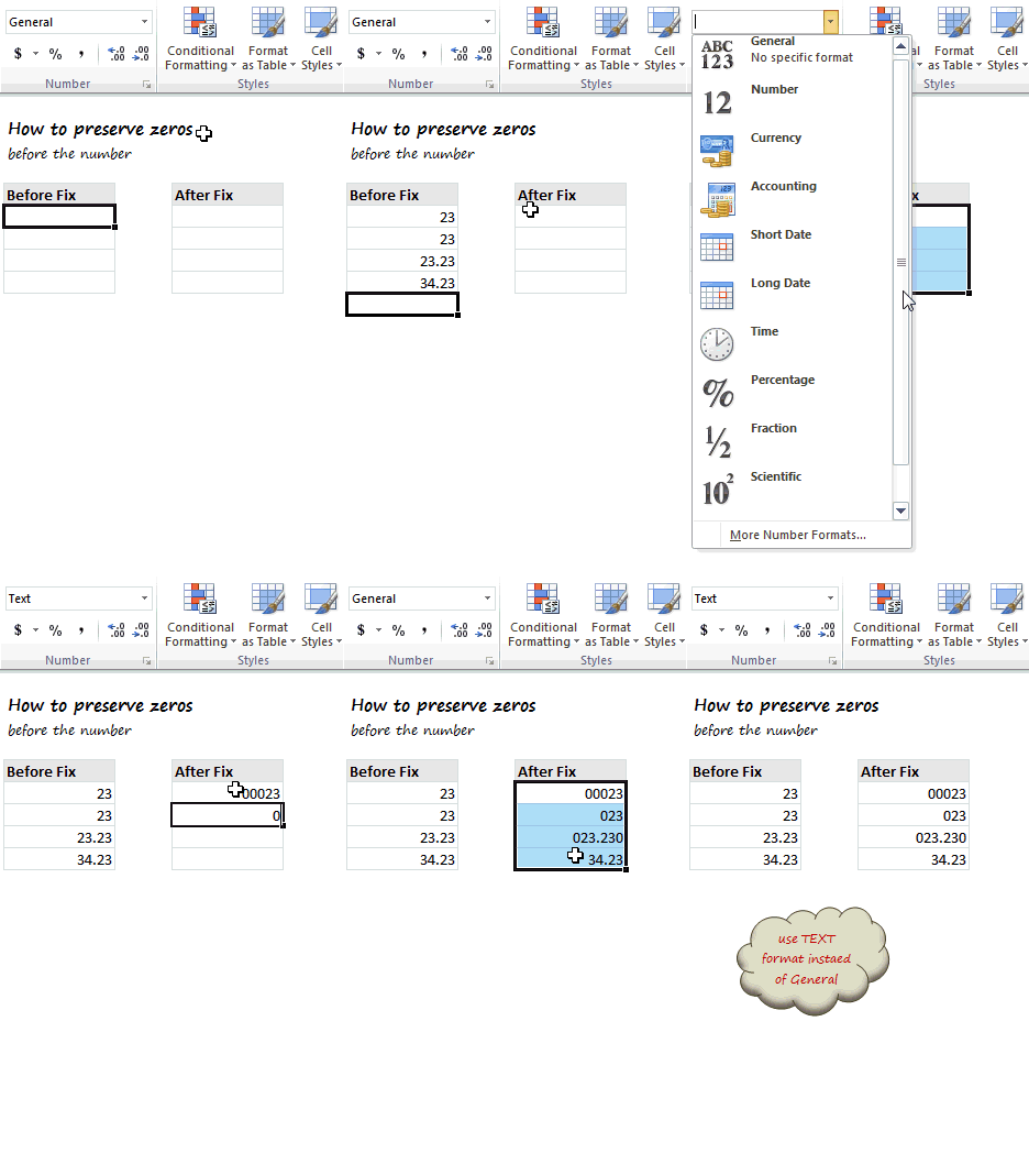
Very simple, we use TEXT format instead of number format. Just select the cells where you are going to enter these numbers, and from Home ribbon > Number area, select “Text” as cell type. This tells Excel to treat any value you enter as Text, not as number. So when you type 00023, it will appear as 00023.
See this short demo to understand how to get this work.
Bonus Tip – Use fixed number of zeros
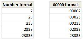 For example, if you want the number to show up in 5 digits (with leading 0s if needed), you can use the cell format code 00000.
To apply this format:
- Just select the cells and press CTRL+1
- From Number tab choose “Custom”
- Enter the format code as
00000 - Done!
Aside, you can see how this formatting works.
That is all for now. Have a great evening then 🙂
More on Cell Formatting
Excel allows you to format cells in myriad ways, some of which may baffle you. But Chandoo.org got your back! We have written several articles to help you master the cell formatting. Read on,
- Formatting Numbers in Excel – an overview
- Custom Cell Formatting in Excel – Tips
- How to show decimal point only for values less than 1
- Show colors in chart labels based on data
- How to hide cell contents in Excel using cell formats
- More on Number Formatting & Cell formatting
PS: We had a minor hiccup with our newsletter. Many of you did not get it for last 7 days. It is fixed now. So you might get one big email from Chandoo.org with all the missed posts.


30 Responses
You could always use a leading ‘ also, of course.
It’s probably best to use the custom number format than formatting as text out using the leading apostrophe. The only exception that comes to mind is if the number is a credit card number. Excel lewis only the first 15 digits, and turns the rest to zeros.
It doesn’t really work, I’m sorry.
After setting the “00000” in custom. The number does change to “00023”. However, if you go back to cell format, it will show up under “Special” -> “Zip Code”. i’m using excel 2007.
Also, I have customer ID that starts with zero from another system. When that ID (along with a table of data) is pulled into Excel it will show as 000023 with a cell format “General”. if you F2 that cell the zeros would be gone so I don’t want to mess with it.
The problem is that you can’t do vlookup between 2 cells one with a zip code format and the other one as General. I have seen that in the past and it won’t work.
I ended up getting a different solution, not smart/efficient but works for me. I enter “000”&23, copy and paste as value on the same cell. This way, the ID 00023 generated by a different system dl to Excel is compatible to other data. To make my life easier I have generated, on the side, a list of customers whose ID start with 0. When I need them, I’ll just pull them to the worksheet where I need them.
Fred –
The problem is not a lookup in different formats, it’s that some of your values are numerical and some text.
Your values that visibly change when you use the 00000 format are numbers. The values that come in from another system with leading zeros, come in as text which preserves the zeros as text. The General format shows the text complete with leading zeros and numbers without any leading zeros and without trailing zeros after the decimal point. F2 makes Excel re-evaluate the numbers, and converts them from text with leading zeros to numbers without.
If it were my data, I’d convert everything to numbers and apply appropriate number formats. Then I wouldn’t have to keep a separate list of special companies, and change my data whenever one of them were involved.
It seems like a really bad idea to suggest using text to preserve leading zeros, particularly in light of all of the concern these days abut spreadsheet integrity and managing risks in spreadsheets.
Very good point. When you are entering numbers, I see no reason why you would want leading zeros. But when you are entering text data (such as customer numbers, invoice numbers, product codes) that looks like numbers, then using TEXT format is actually a better choice since you are not going to sum-up or do other such arithmetic with them.
If a field contains entries that may be numbers or text, then treat the field as text. If the field only contains numbers, I still think you should retain their numerical values and adjust their appearance using number formats.
Beware if doing arithmetic operations to a “Text Number” – =/+ an individual cell will return something meaningfull, SUM() will ignore a non-numeric style and return 0. Prefacing with a ‘ will also generate the same behaviour.
Chandoo, sometimes these numbers are expected in a fixed format.
In where I work, the employee id is always in 7 digits. So in columns that indicate employee id, we always format with Custom 7 digits. this really helps easy reading.
I always use the Custom format rather than the text or using ‘ before the numbers because the latter two cases will not help using any formulas.
Murugaraj, even if the employee ID is stored in a company database as an integer, you’re never going to be treating the ID as a number (such as performing arithmetic on it.) A system I work with has a 10 digit ID that is all numbers, but starts with zeroes in some cases. We always treat these IDs as strings.
One problem I have is that even though they’re strings, exporting CSV from the database results in columns that are treated as numbers and lose the starting zeroes. In this case, I usually add another column with the formula =REPT(0,8-LEN(A1))&A1. This formula will create a column with a string padded with the correct number of zeroes (enough for 8 digits in this example.)
I frequently need to change a list mixed with 3, 4, and 5 digits to uniformly 5 digits by adding leading zeros.
I was excited about the custom format solution, but then I realized the underlying cell value is still 3 or 4 digits, realizing that custom formatting is just that, merely a format applied to a value. If I copy and paste to another location, the 3 or 4 digit values remain.
The other way to write a formula such as =”0″&A1 but I like your method better. Any workaround to make it work in my case?
You could use
=TEXT(A1,”00000″)
which shows a 5-digit number in the cell but treats it as text. Copy and paste deals with the 5-digit text, not the underlying numerical value.
This works for CSV export – Like!
I am a newbie to excel and never got an opportunity to explore much on it. As I started working on it, the results were startling. I am really impressed by the way the site is organized and I am book marking this site as a one stop to my excel problems.
How to format 28,654,124 to show as 28,000,000 using custom formatting (without using round() formula)
@Nelson: If the numbers are always in millions, you can try below custom format code:
#,,”000,000″
If he really wants 28.6 million to appear as 28.0 million instead of 29.0 million, he’ll have to use a formula
Thank You Peltier.
You are right.
My focus was on getting six zeroes. I overlooked.
So nice of you.
Thank You Chandoo.
Highly appreciated.
The output was 29000,000
I changed it to #,,”,000,000″
Thank You.
How to VLOOKUP serial IDs with leading zeros & without zeros
I have an issue when doing sumif functions for items that have leading zero’s. The item numbers in our production facility may or may not have leading zero’s and can match if you drop the leading zero. For example; item number 12399 is not the same item as 012399 if our system. If I am doing a sumif on the item number, even if both items are formatted as text, excel will add the column that I am summing together for both items. If I did a sumif on the info below to get total yearly sales excel will return 10 for both item numbers. this is causing some real issues for me. Does anyone have a solution?
Item Sales Qty Month
‘12399 5 Jan
‘012399 5 Feb
@Rebecca… strange, but you are right. SUMIF(s) would forcefully convert condition values to numbers. You can use SUMPRODUCT in cases like this.
Refer to: http://chandoo.org/wp/2009/11/10/excel-sumproduct-formula/ for an idea on how to use this.
I have tried all your suggestions above…. still can’t get leading zeros back into zip code field that were dropped when I imported a csv file. I saw in the custom format where I could add “0” back in but only to five digits — my zip code field has all 9 digits (zip plus4) all together
Example1: 9digit Zip code field for Puerto Rico After import: 6105458
should be: 006055132
Example 2: 9 digit Zip code field for MA After import: 19601714
should be 019601714
I tried all of the suggestions above – can’t get anything to work — any other suggestions – or ideas what I am doing wrong?
If you have your ZIP-code in cell A1, you could try the following formula in cell B1 =IF(LEN(A1)<9;REPT("0";9-LEN(A1))&A1;A1)
I know this is a poor work-around 🙁
God bless you real good, you just saved someone’s ass in ma office !
I was trying to add zero in my excel but it’s not happening. I was quite frustrated and i start searching the way to do it and luckily i got this page. I have did according to your described way and it’s working. Thanks for sharing such a valuable resource.
B
7
8
7
3
1
9
7
8
7
4
I have this column and I am used this formule
=IF(ISNA(VLOOKUP(ROW(B1),$B$1:$B$21,1,FALSE)),ROW(B1),””)
0
2
5
6
10
I need include the zero , but i have only 2, 5, 6, 10.
Can you help me? Please.
Hi,
what format should I use if the cell contains a formula?
If I use text it doesn’t resolve the formula but displays it instead.
I need the last two digit of the decimal, Eg: 1425.50 or 1425.00 then I have to get 50 or 00. I tried this this formula but zero is not getting.=IF(IFERROR(FIND(“.”,B129:B129),0)>0,MID(B129:B129,FIND(“.”,B129:B129)+1,99),””)
i have a list of phone nos i copied from word to excell all starting with zero but the leading zero doesn’t appear . what do i do